Chapter 08 – Index Models
CHAPTER 8: INDEX MODELS
PROBLEM SETS
1. The advantage of the index model, compared to the Markowitz procedure, is the vastly
reduced number of estimates required. In addition, the large number of estimates
2. The trade-off entailed in departing from pure indexing in favor of an actively managed
3. The answer to this question can be seen from the formulas for w 0 and w*. Other things
held equal, w 0 is smaller the greater the residual variance of a candidate asset for
inclusion in the portfolio. Further, we see that regardless of beta, when w 0 decreases, so
4. The total risk premium equals: + ( × market risk premium). We call alpha a
“nonmarket” return premium because it is the portion of the return premium that is
independent of market performance.
The Sharpe ratio indicates that a higher alpha makes a security more desirable. Alpha,
the numerator of the Sharpe ratio, is a fixed number that is not affected by the standard
8-2
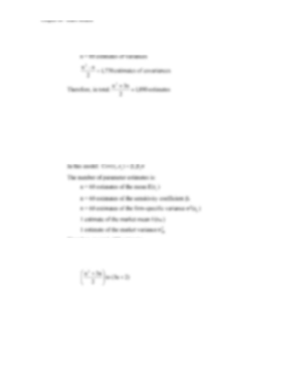
5. a. To optimize this portfolio one would need:
n = 60 estimates of means
2
b. In a single index model: ri − rf = i + i (r M – rf ) + e i
Equivalently, using excess returns: R i = i + i R M + e i
The variance of the rate of return on each stock can be decomposed into the
components:
(l) The variance due to the common market factor:
2
M
2
i
(2) The variance due to firm specific unanticipated events:
)e( i
2
M
Therefore, in total, 182 estimates.
Thus, the single index model reduces the total number of required parameter
estimates from 1,890 to 182. In general, the number of parameter estimates is
reduced from:
)2n3( to
2
n3n2+
+
Chapter 08 – Index Models
6. a. The standard deviation of each individual stock is given by:
2/1
i
22
M
2
ii )]e([ +=
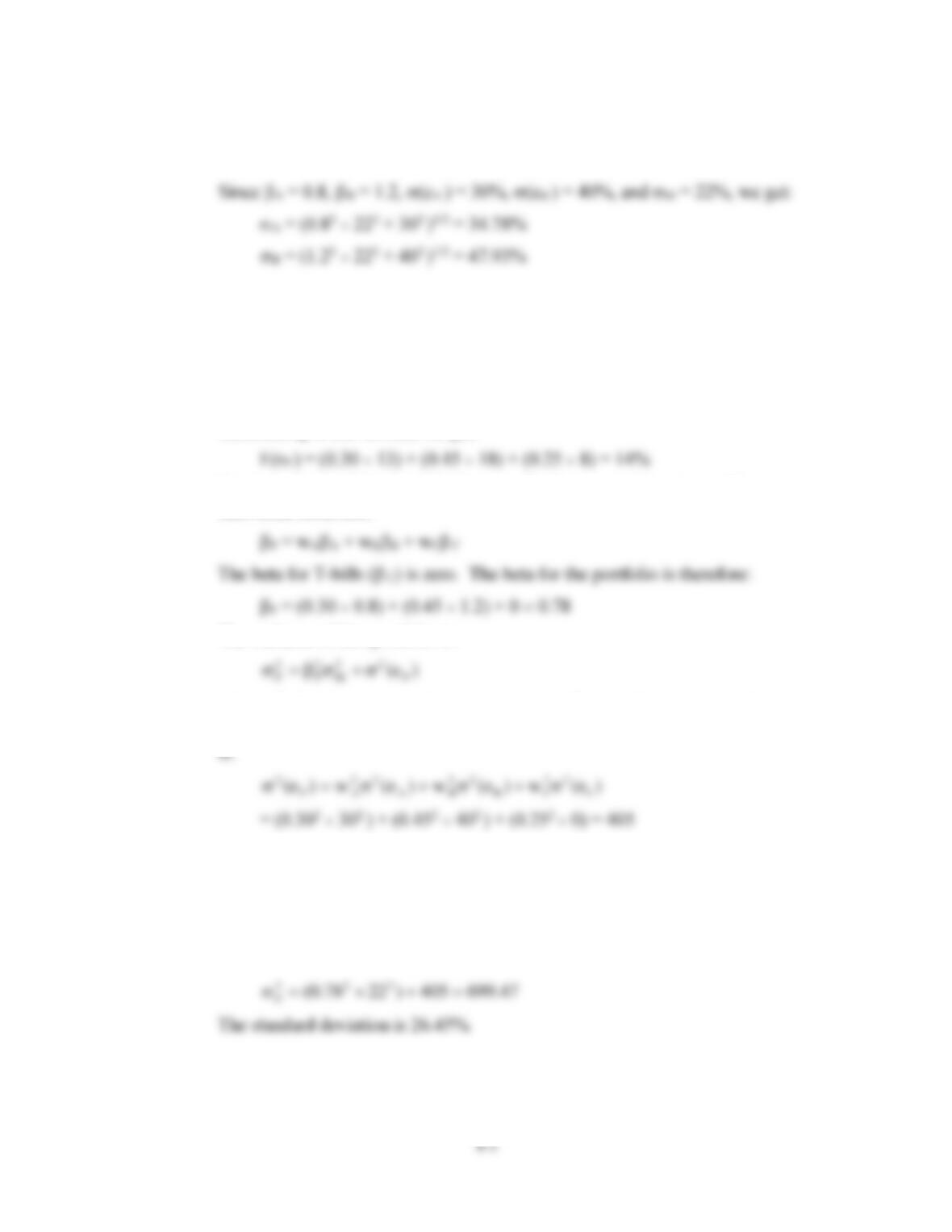
b. The expected rate of return on a portfolio is the weighted average of the expected
returns of the individual securities:
E(rP ) = wAE(rA ) + wBE(rB ) + wf rf
where wA , wB , and wf are the portfolio weights for Stock A, Stock B, and T-
bills, respectively.
Substituting in the formula we get:
The beta of a portfolio is similarly a weighted average of the betas of the
individual securities:
The variance of this portfolio is:
)e( P
22
M
2
P
2
P+=
where
2
M
2
P
is the systematic component and
)e( P
2
is the nonsystematic
component. Since the residuals (ei ) are uncorrelated, the non-systematic variance
where 2(eA ) and 2(eB ) are the firm-specific (nonsystematic) variances of
Stocks A and B, and 2(e f ), the nonsystematic variance of T-bills, is zero. The
residual standard deviation of the portfolio is thus:
(e P ) = (405)1/2 = 20.12%
The total variance of the portfolio is then:
47.699405)2278.0( 222
P=+=
The standard deviation is 26.45%.
8-4
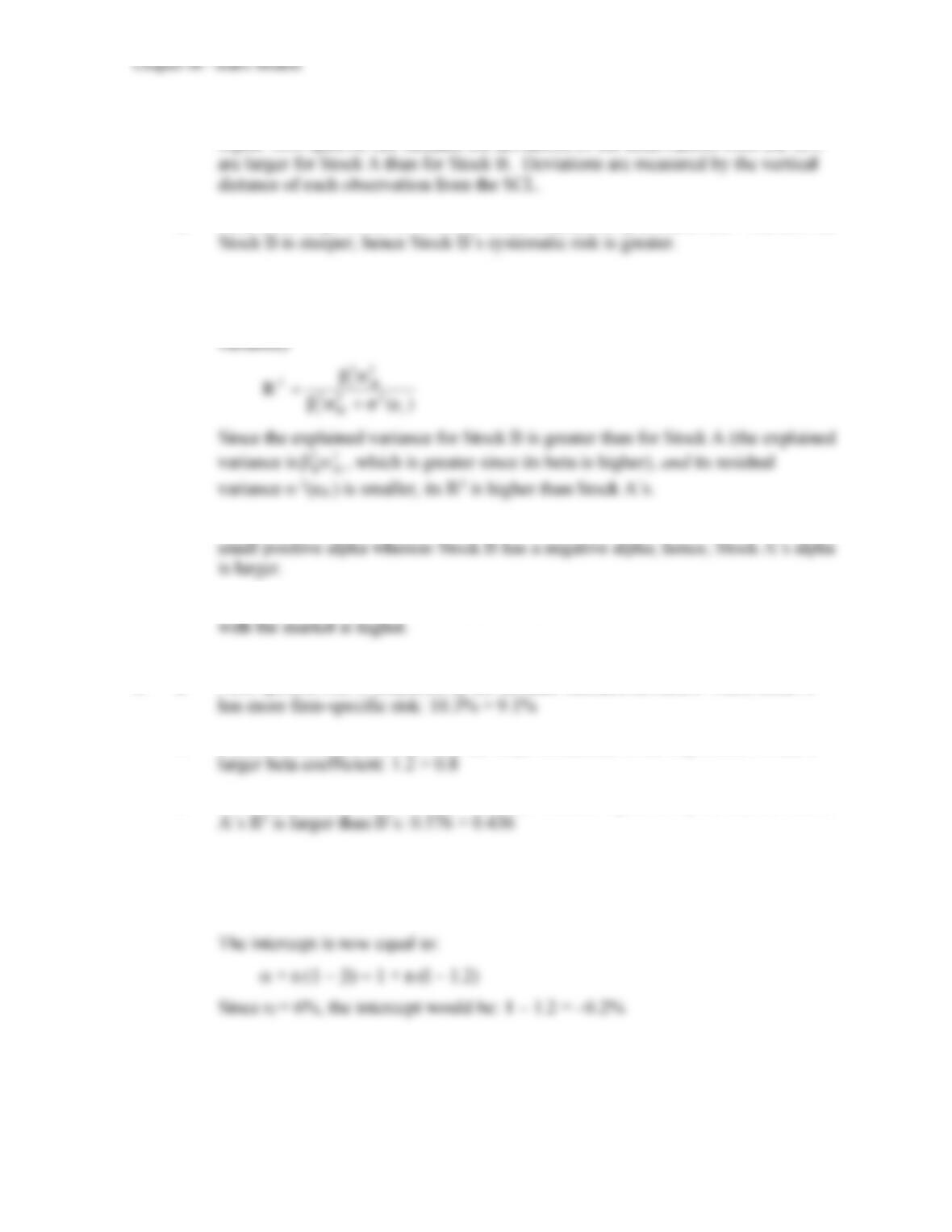
7. a. The two figures depict the stocks’ security characteristic lines (SCL). Stock A has
higher firm-specific risk because the deviations of the observations from the SCL
b. Beta is the slope of the SCL, which is the measure of systematic risk. The SCL for
c. The R2 (or squared correlation coefficient) of the SCL is the ratio of the explained
variance of the stock’s return to total variance, and the total variance is the sum of
the explained variance plus the unexplained variance (the stock’s residual
d. Alpha is the intercept of the SCL with the expected return axis. Stock A has a
e. The correlation coefficient is simply the square root of R2, so Stock B’s correlation
8. a. Firm-specific risk is measured by the residual standard deviation. Thus, stock A
b. Market risk is measured by beta, the slope coefficient of the regression. A has a
c. R2 measures the fraction of total variance of return explained by the market return.
d. Rewriting the SCL equation in terms of total return (r) rather than excess return
(R):
rA – rf = + (rM – rf ) rA = + rf (1 − ) + r M
Chapter 08 – Index Models
8-5
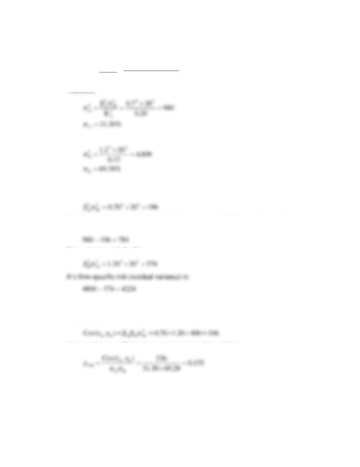
9. The standard deviation of each stock can be derived from the following equation
for R2:
=
=2
i
2
M
2
i
2
i
R
Explained variance
Total variance
%30.31
A
A
=
For stock B:
%28.69
800,4
12.0
202.1
B
22
2
B
=
=
=
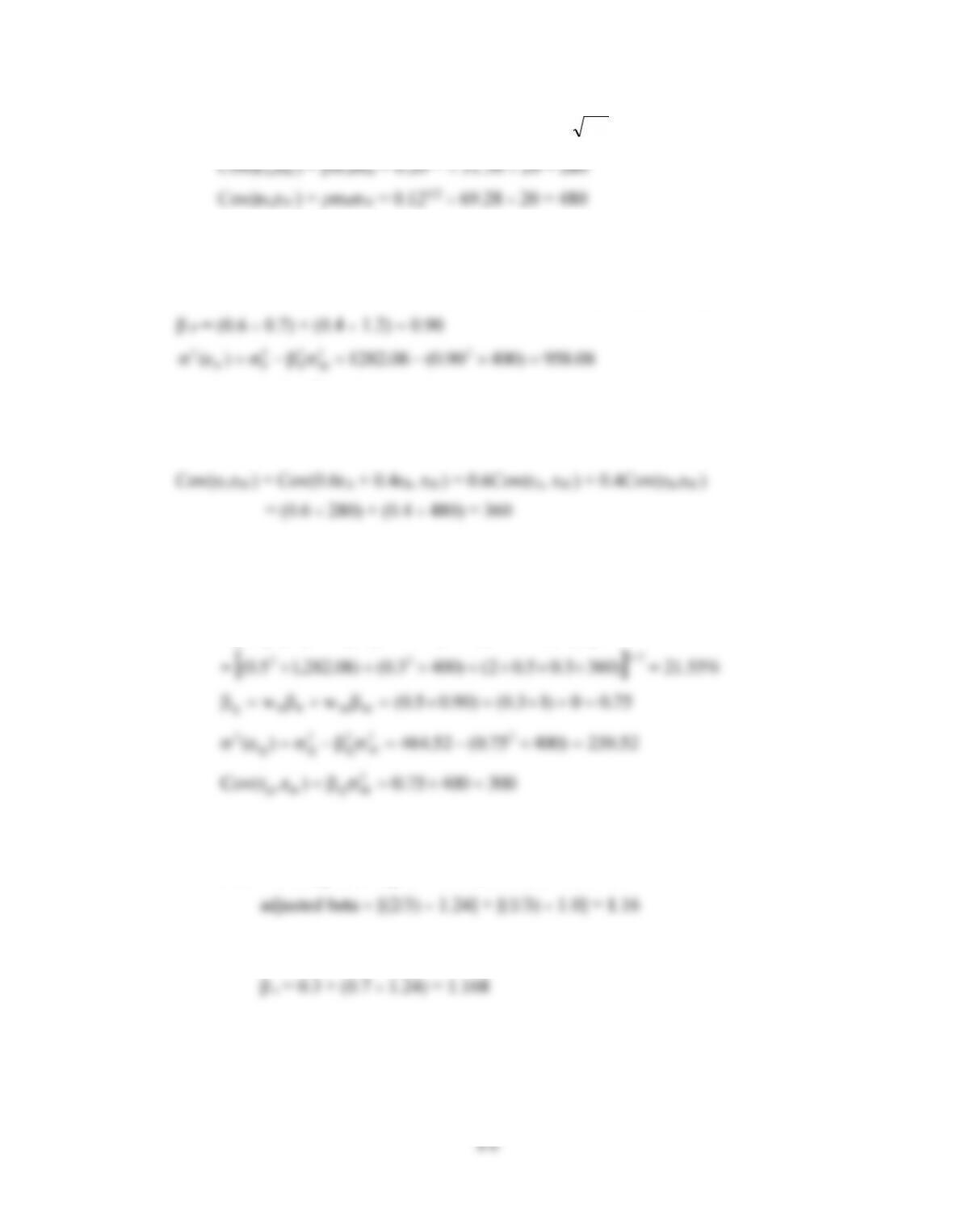
10. The systematic risk for A is:
1962070.0 222
M
2
A==
The firm-specific risk of A (the residual variance) is the difference between A’s
total risk and its systematic risk:
The systematic risk for B is:
5762020.1 222
M
2
B==
B’s firm-specific risk (residual variance) is:
4800 – 576 = 4224
11. The covariance between the returns of A and B is (since the residuals are assumed to be
uncorrelated):
33640020.170.0)r,r(Cov 2
MBABA ===
The correlation coefficient between the returns of A and B is:
155.0
28.6930.31
336
)r,r(Cov
BA
BA
AB =
=
=
Chapter 08 – Index Models
12. Note that the correlation is the square root of R2:
2
R=
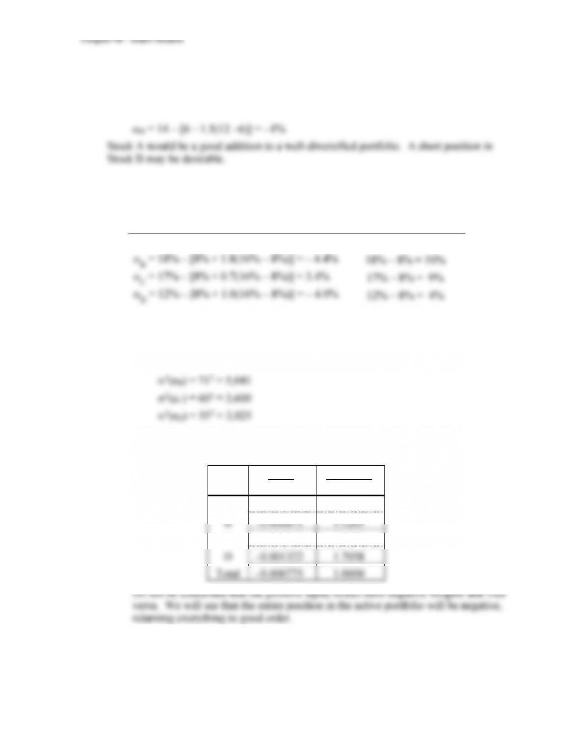
13. For portfolio P we can compute:
P = [(0.62 980) + (0.42 4800) + (2 0.4 0.6 336]1/2 = [1282.08]1/2 = 35.81%
M
P
PP
Cov(rP,rM ) = P
2
M
σ
=0.90 × 400=360
This same result can also be attained using the covariances of the individual stocks with
the market:
14. Note that the variance of T-bills is zero, and the covariance of T-bills with any asset is
zero. Therefore, for portfolio Q:
)r,r(Covww2ww
2/1
MPMP
2
M
2
M
2
P
2
PQ
++=
MQMQ ===
15. a. Merrill Lynch adjusts beta by taking the sample estimate of beta and averaging it
with 1.0, using the weights of 2/3 and 1/3, as follows:
b. If you use your current estimate of beta to be t–1 = 1.24, then
8-7
16. For Stock A:
A = rA − rf + A(rM −rf )] = 11 − [6 +0.8(12 − 6)] = 0.2%
For stock B:
17. a.
Alpha ()
Expected excess return
i = ri – [rf + i(rM – rf ) ]
E(ri ) – rf
A = 20% – [8% + 1.3(16% – 8%)] = 1.6%
20% – 8% = 12%
B = 18% – [8% + 1.8(16% – 8%)] = – 4.4%
18% – 8% = 10%
C = 17% – [8% + 0.7(16% – 8%)] = 3.4%
17% – 8% = 9%
D = 12% – [8% + 1.0(16% – 8%)] = – 4.0%
12% – 8% = 4%
Stocks A and C have positive alphas, whereas stocks B and D have negative
alphas.
The residual variances are:
2(eA ) = 582 = 3,364
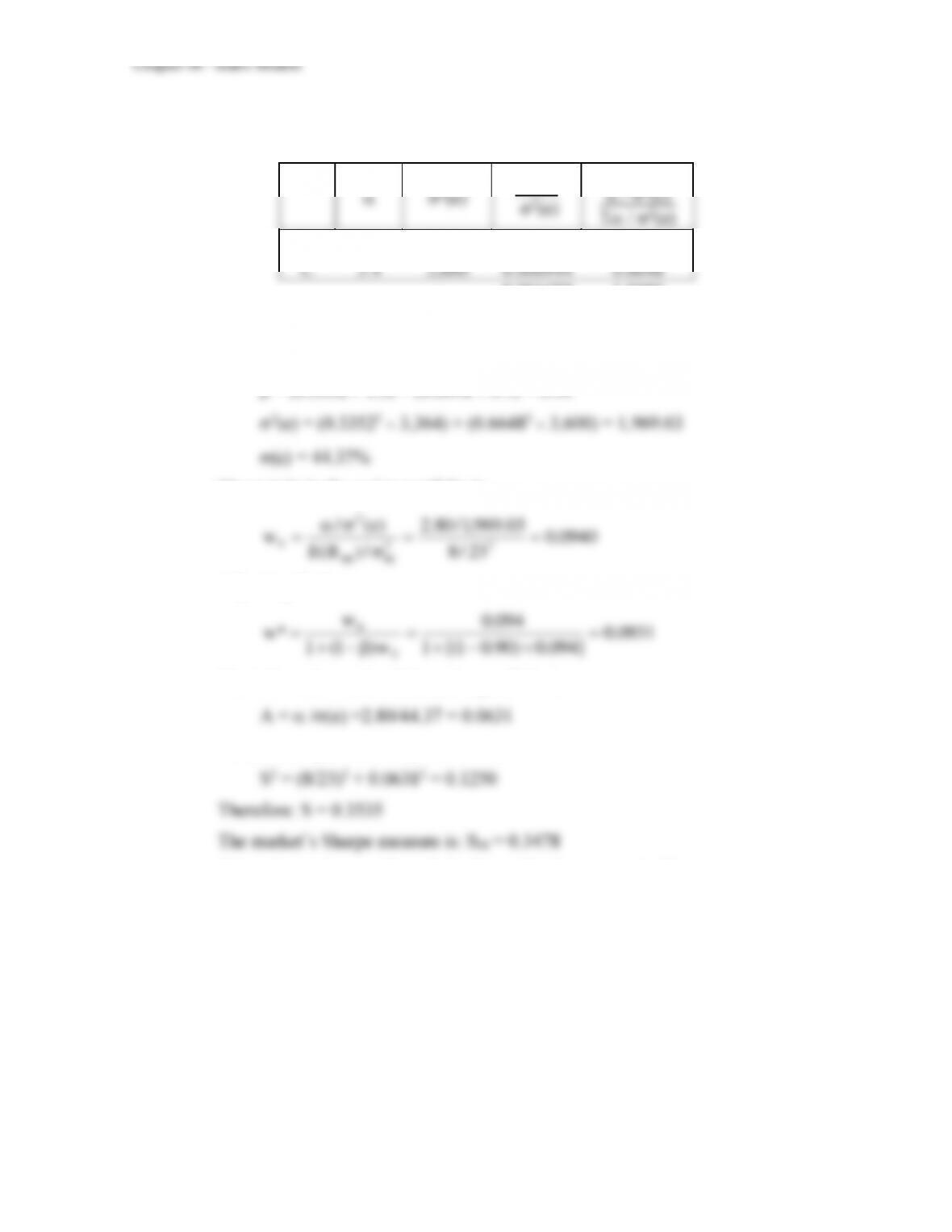
b. To construct the optimal risky portfolio, we first determine the optimal active portfolio.
Using the Treynor-Black technique, we construct the active portfolio:
2(e)
/ 2(e)
2(e)
A
0.000476
–0.6142
B
–0.000873
1.1265
C
0.000944
–1.2181
D
–0.001322
1.7058
Total
–0.000775
1.0000

Chapter 08 – Index Models
8-8
With these weights, the forecast for the active portfolio is:
= [–0.6142 1.6] + [1.1265 (– 4.4)] – [1.2181 3.4] + [1.7058 (– 4.0)]
= –16.90%
The high beta (higher than any individual beta) results from the short positions in
the relatively low beta stocks and the long positions in the relatively high beta
stocks.
2(e) = [(–0.6142)2 3364] + [1.12652 5041] + [(–1.2181)2 3600] + [1.70582 3025]
Here, again, the levered position in stock B [with high 2(e)] overcomes the
diversification effect, and results in a high residual standard deviation. The
optimal risky portfolio has a proportion w* in the active portfolio, computed as
follows:
05124.0
23/8
6.809,21/90.16
/]r)r(E[
)e(/
w22
MfM
2
0−=
−
=
−
=
The negative position is justified for the reason stated earlier.
The adjustment for beta is:
0486.0
)05124.0)(08.21(1
05124.0
w)1(1
w
*w
0
0−=
−−+
−
=
−+
=
Since w* is negative, the result is a positive position in stocks with positive alphas
and a negative position in stocks with negative alphas. The position in the index
portfolio is:
c. To calculate Sharpe’s measure for the optimal risky portfolio, we compute the
information ratio for the active portfolio and Sharpe’s measure for the market portfolio.
The information ratio for the active portfolio is computed as follows:
A = /(e)= –16.90/147.68 = –0.1144
Hence, the square of Sharpe’s measure (S) of the optimized risky portfolio is:
1341.00131.0
23
8
ASS
2
22
M
2=+
=+=

Chapter 08 – Index Models
Compare this to the market’s Sharpe measure:
SM = 8/23 = 0.3478
The difference is: 0.0184
d. To calculate the exact makeup of the complete portfolio, we first compute `the
mean excess return of the optimal risky portfolio and its variance. The risky
portfolio beta is given by:
P = wM + (wA A ) = 1.0486 + [(–0.0486) 2.08] = 0.95
E(RP) = P + PE(RM) = [(–0.0486) (–16.90%)] + (0.95 8%) = 8.42%
( )
94.5286.809,21)0486.0()2395.0()e( 22
P
22
M
2
P
2
P=−+=+=
%00.23
P=
Since A = 2.8, the optimal position in this portfolio is:
5685.0
94.5288.201.0
42.8
y=
=
In contrast, with a passive strategy:
5401.0
238.201.0
8
y2=
=
This is a difference of: 0.0284
The final positions of the complete portfolio are:
Bills
1 – 0.5685 =
43.15%
M
0.5685 l.0486 =
59.61%
A
0.5685 (–0.0486) (–0.6142) =
1.70%
B
0.5685 (–0.0486) 1.1265 =
– 3.11%
C
0.5685 (–0.0486) (–1.2181) =
3.37%
D
0.5685 (–0.0486) 1.7058 =
– 4.71%
100.00%
[sum is subject to rounding error]
Note that M may include positive proportions of stocks A through D.
8-10
18. a. If a manager is not allowed to sell short he will not include stocks with negative
alphas in his portfolio, so he will consider only A and C:
2(e)
2(e)
/ 2(e)
2(e)
A
1.6
3,364
0.000476
0.3352
C
3.4
3,600
0.000944
0.6648
0.001420
1.0000
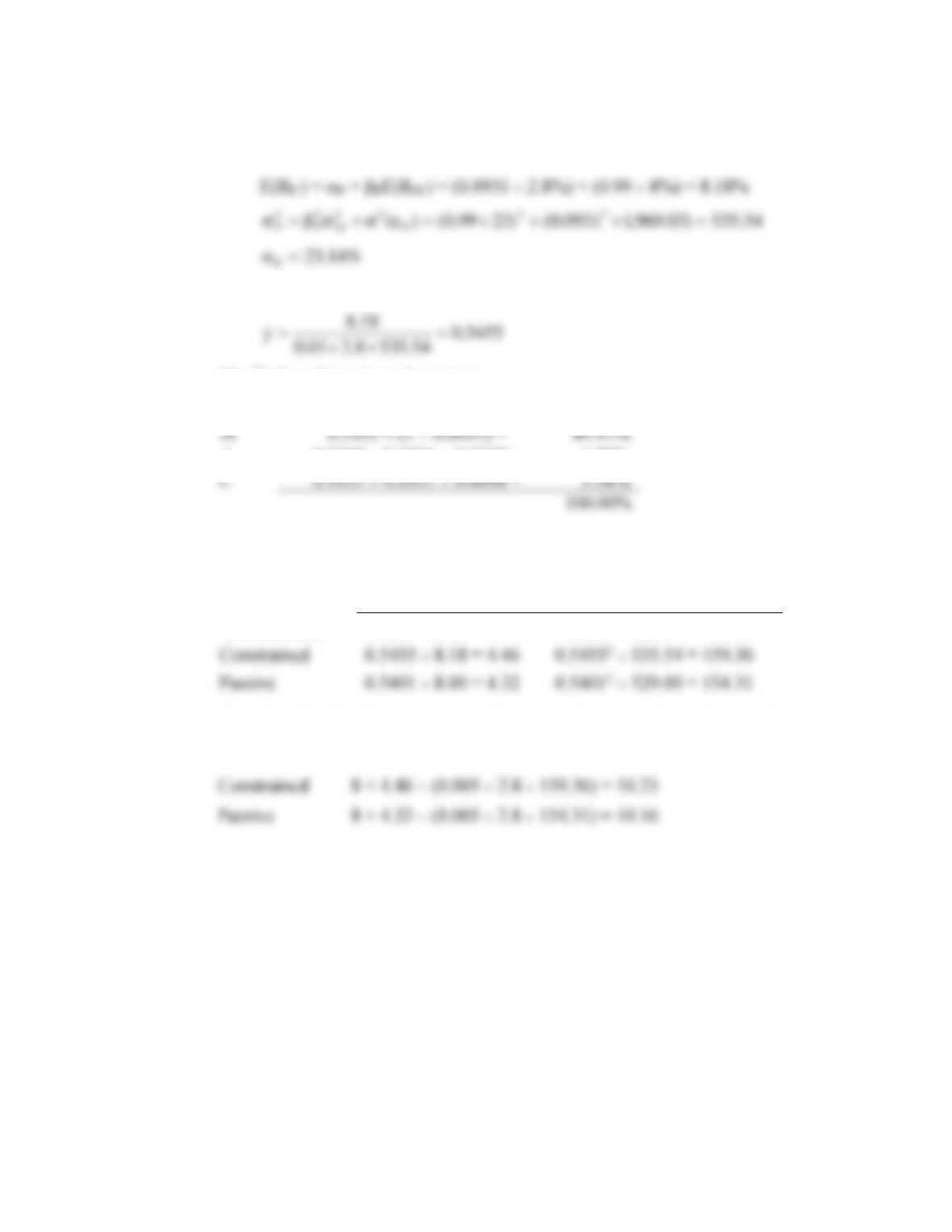
The forecast for the active portfolio is:
= (0.3352 1.6) + (0.6648 3.4) = 2.80%
= (0.3352 1.3) + (0.6648 0.7) = 0.90
The weight in the active portfolio is:
0940.0
23/8
03.969,1/80.2
/)R(E
)e(/
w22
MM
2
0==
=
Adjusting for beta:
0931.0
]094.0)90.01[(1
094.0
w)1(1
w
*w
0
0=
−+
=
−+
=
The information ratio of the active portfolio is:
Hence, the square of Sharpe’s measure is:
When short sales are allowed (Problem 18), the manager’s Sharpe measure is
higher (0.3662). The reduction in the Sharpe measure is the cost of the short sale
restriction.
Chapter 08 – Index Models
8-11
The characteristics of the optimal risky portfolio are:
P = wM + wA A = (1 – 0.0931) + (0.0931 0.9) = 0.99
P=
With A = 2.8, the optimal position in this portfolio is:
5455.0
54.5358.201.0
18.8
y=
=
The final positions in each asset are:
Bills
1 – 0.5455 =
45.45%
M
0.5455 (1 − 0.0931) =
49.47%
A
0.5455 0.0931 0.3352 =
1.70%
C
0.5455 0.0931 0.6648 =
3.38%
100.00%
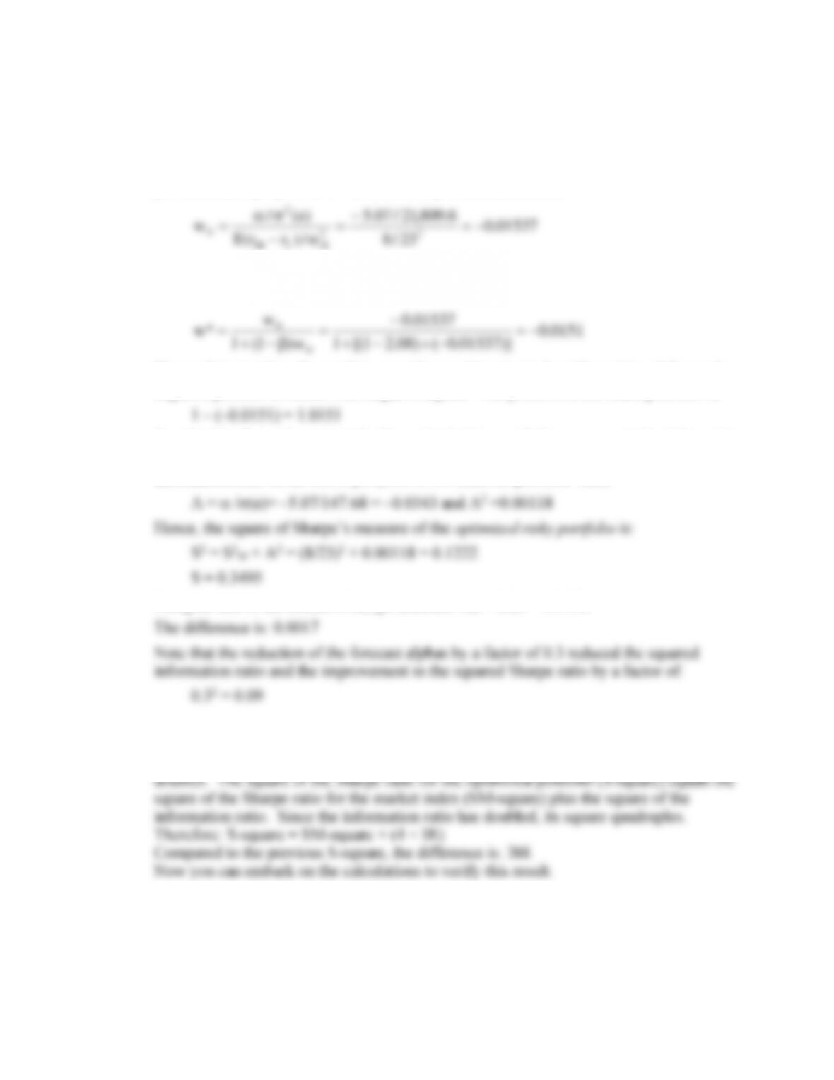
b. The mean and variance of the optimized complete portfolios in the unconstrained
and short-sales constrained cases, and for the passive strategy are:
E(RC )
2
C
Unconstrained
0.5685 8.42 = 4.79
0.56852 528.94 = 170.95
Constrained
0.5455 8.18 = 4.46
0.54552 535.54 = 159.36
Passive
0.5401 8.00 = 4.32
0.54012 529.00 = 154.31
The utility levels below are computed using the formula:
2
CC A005.0)r(E −
Unconstrained 8 + 4.79 – (0.005 2.8 170.95) = 10.40
Chapter 08 – Index Models
8-12
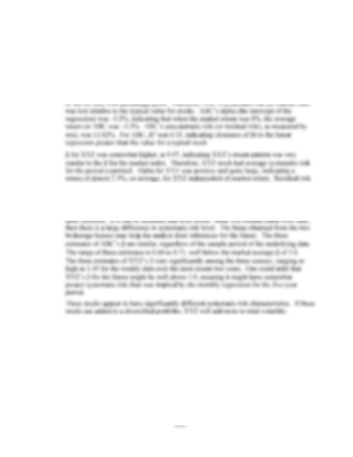
19. All alphas are reduced to 0.3 times their values in the original case. Therefore, the
relative weights of each security in the active portfolio are unchanged, but the alpha of
the active portfolio is only 0.3 times its previous value: 0.3 −16.90% = −5.07%
The investor will take a smaller position in the active portfolio. The optimal risky
portfolio has a proportion w* in the active portfolio as follows:
01537.0
23/8
6.809,21/07.5
/)rr(E
)e(/
w22
MfM
2
0−=
−
=
−
=
The negative position is justified for the reason given earlier.
The adjustment for beta is:
0151.0
)]01537.0()08.21[(1
01537.0
w)1(1
w
*w
0
0−=
−−+
−
=
−+
=
Since w* is negative, the result is a positive position in stocks with positive alphas and a
negative position in stocks with negative alphas. The position in the index portfolio is:
To calculate Sharpe’s measure for the optimal risky portfolio we compute the information
ratio for the active portfolio and Sharpe’s measure for the market portfolio. The
information ratio of the active portfolio is 0.3 times its previous value:
Compare this to the market’s Sharpe measure: SM = 8/23 = 0.3478
20. If each of the alpha forecasts is doubled, then the alpha of the active portfolio will also
double. Other things equal, the information ratio (IR) of the active portfolio also
Chapter 08 – Index Models
CFA PROBLEMS
1. The regression results provide quantitative measures of return and risk based on monthly
returns over the five-year period.
for ABC was 0.60, considerably less than the average stock’s of 1.0. This indicates
that, when the S&P 500 rose or fell by 1 percentage point, ABC’s return on average rose
was 21.45%, half again as much as ABC’s, indicating a wider scatter of observations
around the regression line for XYZ. Correspondingly, the fit of the regression model
was considerably less than that of ABC, consistent with an R2 of only 0.17.
The effects of including one or the other of these stocks in a diversified portfolio may be
8-14
2. The R2 of the regression is: 0.702 = 0.49