Chapter 7 – Optimal Risky Portfolios
CHAPTER 7: OPTIMAL RISKY PORTFOLIOS
PROBLEM SETS
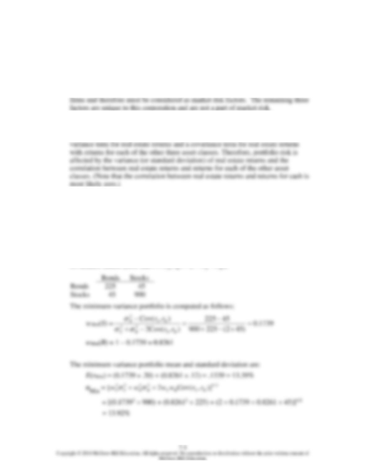
1. (a) and (e). Short-term rates and labor issues are factors that are common to all
2. (a) and (c). After real estate is added to the portfolio, there are four asset classes in
the portfolio: stocks, bonds, cash, and real estate. Portfolio variance now includes a
3. (a) Answer (a) is valid because it provides the definition of the minimum variance
portfolio.
4. The parameters of the opportunity set are:
E(rS) = 20%, E(rB) = 12%, σS = 30%, σB = 15%, ρ = 0.10
From the standard deviations and the correlation coefficient we generate the
covariance matrix [note that
( , )
Cov r r
=
]:
Chapter 7 – Optimal Risky Portfolios
7-2
5.
Proportion
in Stock Fund
Proportion
in Bond Fund
Expected
Return
Standard
Deviation
0.00%
100.00%
12.00%
15.00%
20.00
80.00
40.00
60.00
60.00
40.00
80.00
20.00
Graph shown below.
10.00
15.00
20.00
25.00
Tangency
CML
INVESTMENT OPPORTUNITY SET
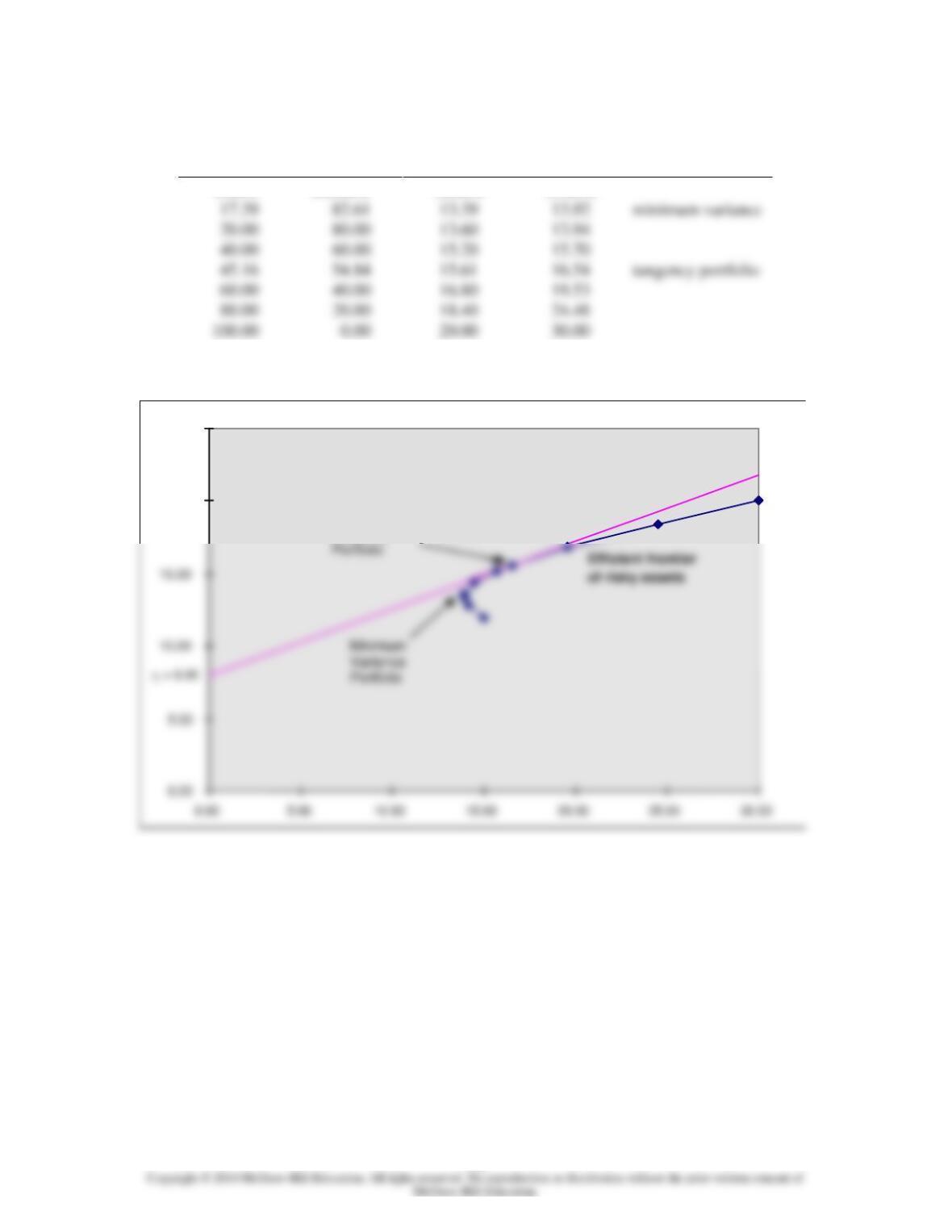
6. The above graph indicates that the optimal portfolio is the tangency portfolio with
expected return approximately 15.6% and standard deviation approximately 16.5%.
Chapter 7 – Optimal Risky Portfolios
7-3
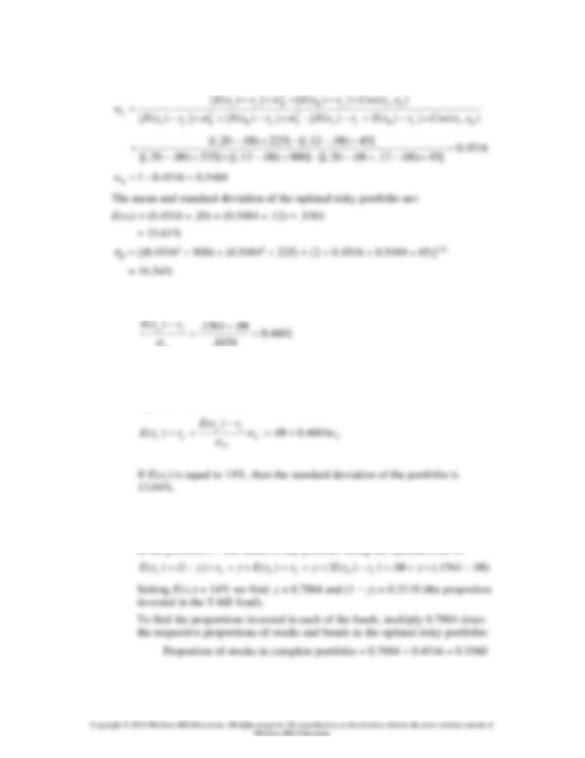
7. The proportion of the optimal risky portfolio invested in the stock fund is given by:
8. The reward-to-volatility ratio of the optimal CAL is:
p
9. a. If you require that your portfolio yield an expected return of 14%, then you
can find the corresponding standard deviation from the optimal CAL. The
equation for this CAL is:
b. To find the proportion invested in the T-bill fund, remember that the mean of
the complete portfolio (i.e., 14%) is an average of the T-bill rate and the
optimal combination of stocks and bonds (P). Let y be the proportion invested
in the portfolio P. The mean of any portfolio along the optimal CAL is:
Chapter 7 – Optimal Risky Portfolios
7-4
10. Using only the stock and bond funds to achieve a portfolio expected return of 14%,
we must find the appropriate proportion in the stock fund (wS) and the appropriate
proportion in the bond fund (wB = 1 − wS) as follows:
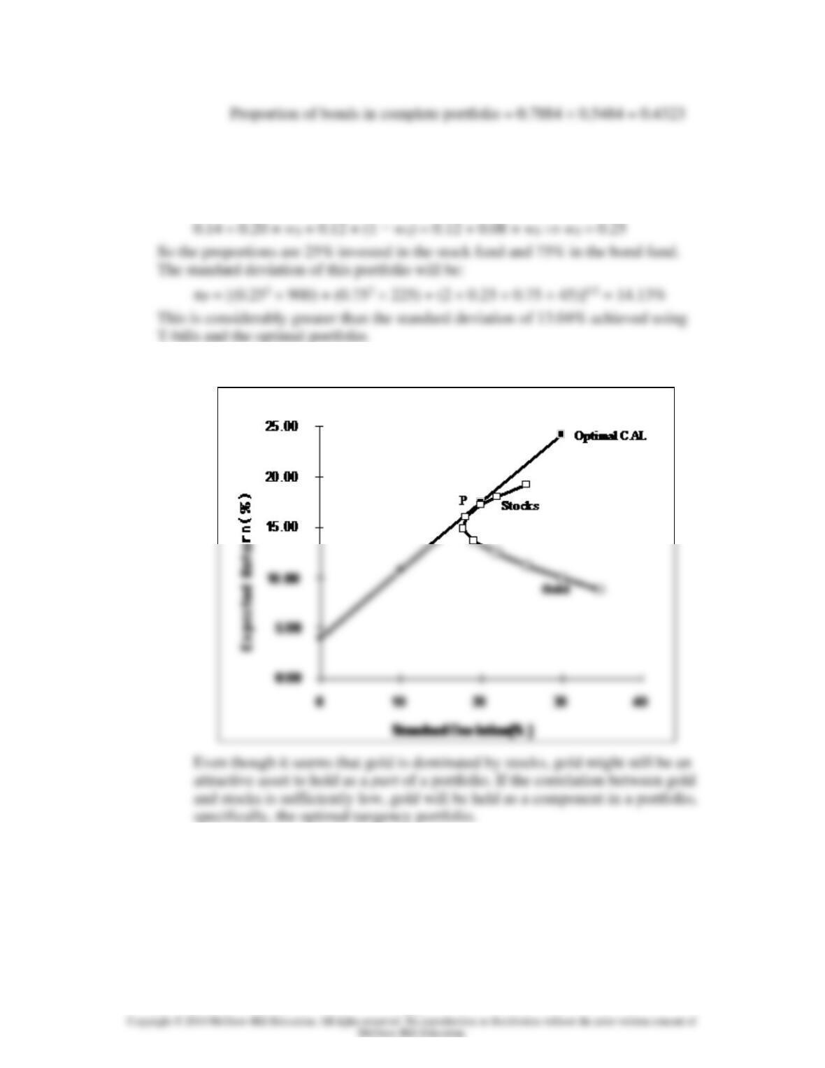
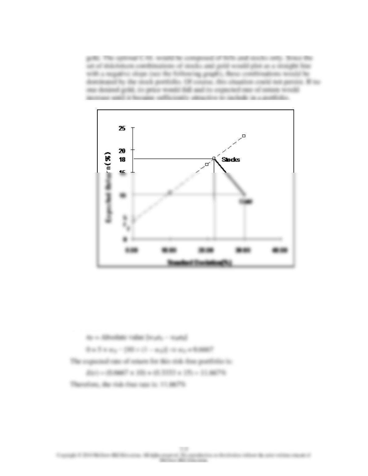
11. a.
Chapter 7 – Optimal Risky Portfolios
b. If the correlation between gold and stocks equals +1, then no one would hold
12. Since Stock A and Stock B are perfectly negatively correlated, a risk-free portfolio
can be created and the rate of return for this portfolio, in equilibrium, will be the
risk-free rate. To find the proportions of this portfolio [with the proportion wA
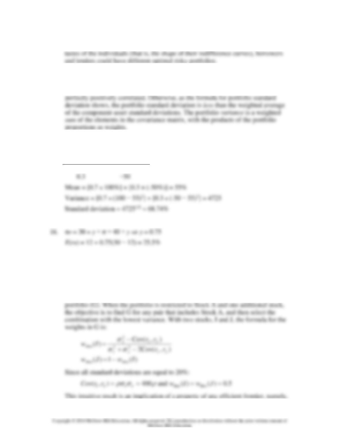
invested in Stock A and wB = (1 – wA ) invested in Stock B], set the standard
deviation equal to zero. With perfect negative correlation, the portfolio standard
deviation is:
Chapter 7 – Optimal Risky Portfolios
7-6
13. False. If the borrowing and lending rates are not identical, then, depending on the
14. False. The portfolio standard deviation equals the weighted average of the
component-asset standard deviations only in the special case that all assets are
15. The probability distribution is:
Probability
Rate of Return
0.7
100%
0.3
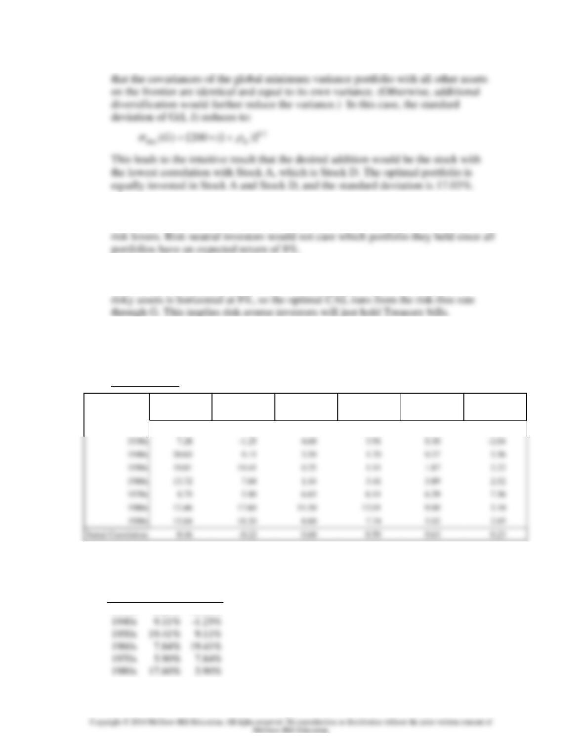
17. The correct choice is (c). Intuitively, we note that since all stocks have the same
expected rate of return and standard deviation, we choose the stock that will result
in lowest risk. This is the stock that has the lowest correlation with Stock A.
More formally, we note that when all stocks have the same expected rate of return,
the optimal portfolio for any risk-averse investor is the global minimum variance
Chapter 7 – Optimal Risky Portfolios
7-7
18. No, the answer to Problem 17 would not change, at least as long as investors are not
19. Yes, the answers to Problems 17 and 18 would change. The efficient frontier of
20. Rearrange the table (converting rows to columns) and compute serial correlation
results in the following table:
Nominal Rates
Small
Company
Stocks
Large
Company
Stocks
Long-Term
Government
Bonds
Intermed-Term
Government
Bonds
Treasury
Bills
Inflation
1920s
-3.72
18.36
3.98
3.77
3.56
-1.00
For example: to compute serial correlation in decade nominal returns for large-
company stocks, we set up the following two columns in an Excel spreadsheet.
Then, use the Excel function “CORREL” to calculate the correlation for the data.
Decade
Previous
1930s
-1.25%
18.36%
1960s
19.41%
Chapter 7 – Optimal Risky Portfolios
7-8
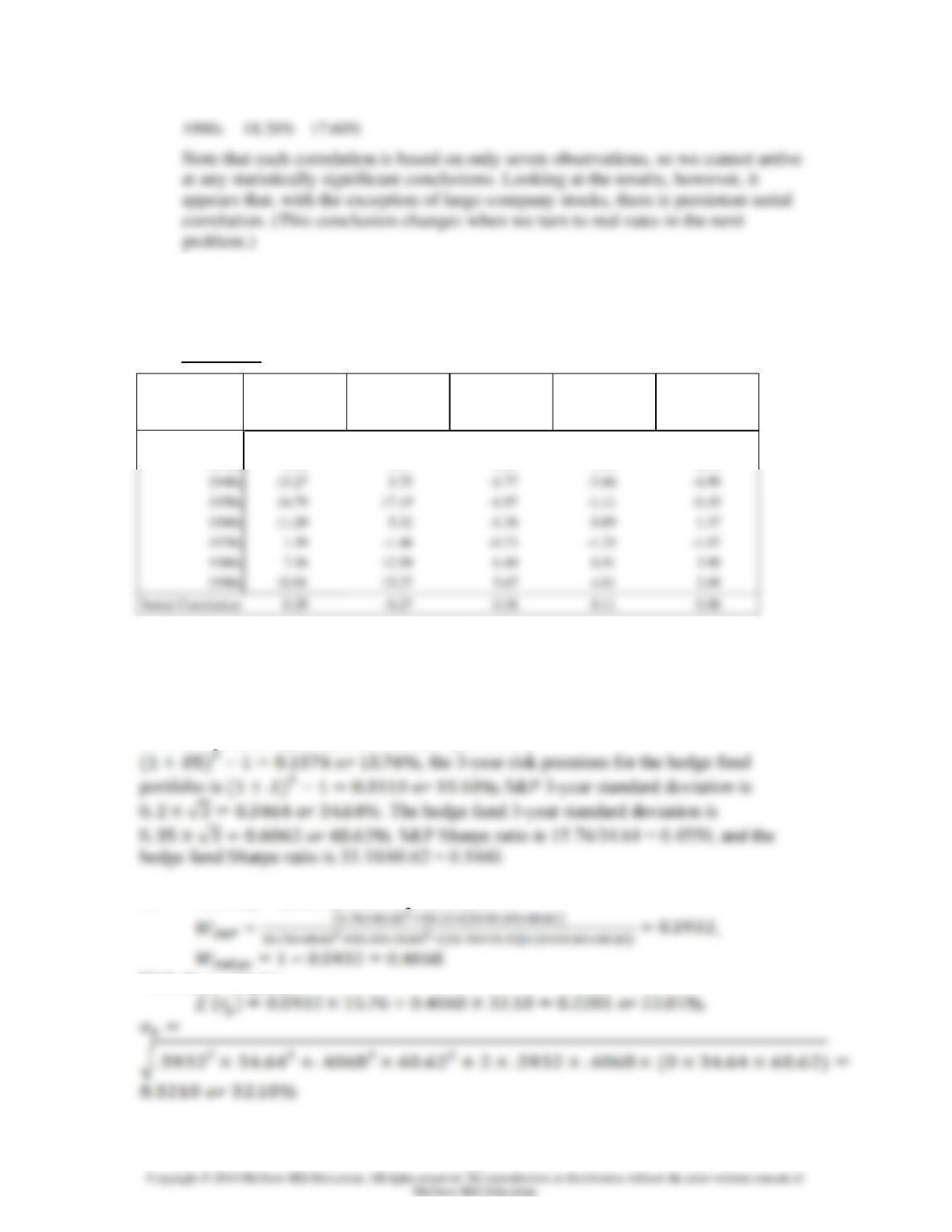
21. The table for real rates (using the approximation of subtracting a decade’s average
inflation from the decade’s average nominal return) is:
Real Rates
Small
Company
Stocks
Large
Company
Stocks
Long-Term
Government
Bonds
Intermed-Term
Government
Bonds
Treasury
Bills
1920s
-2.72
19.36
4.98
4.77
4.56
1930s
9.32
0.79
6.64
5.95
2.34
1950s
16.79
17.19
-1.97
-1.11
-0.35
1960s
11.20
5.32
-1.38
0.89
1.37
1980s
7.36
12.50
6.40
6.91
3.90
1990s
10.91
15.27
5.67
4.81
2.09
0.29
-0.27
0.38
0.11
0.00
While the serial correlation in decade nominal returns seems to be positive, it
appears that real rates are serially uncorrelated. The decade time series (although
again too short for any definitive conclusions) suggest that real rates of return are
independent from decade to decade.
22. The 3-year risk premium for the S&P portfolio is
23. With a ρ = 0, the optimal asset allocation is
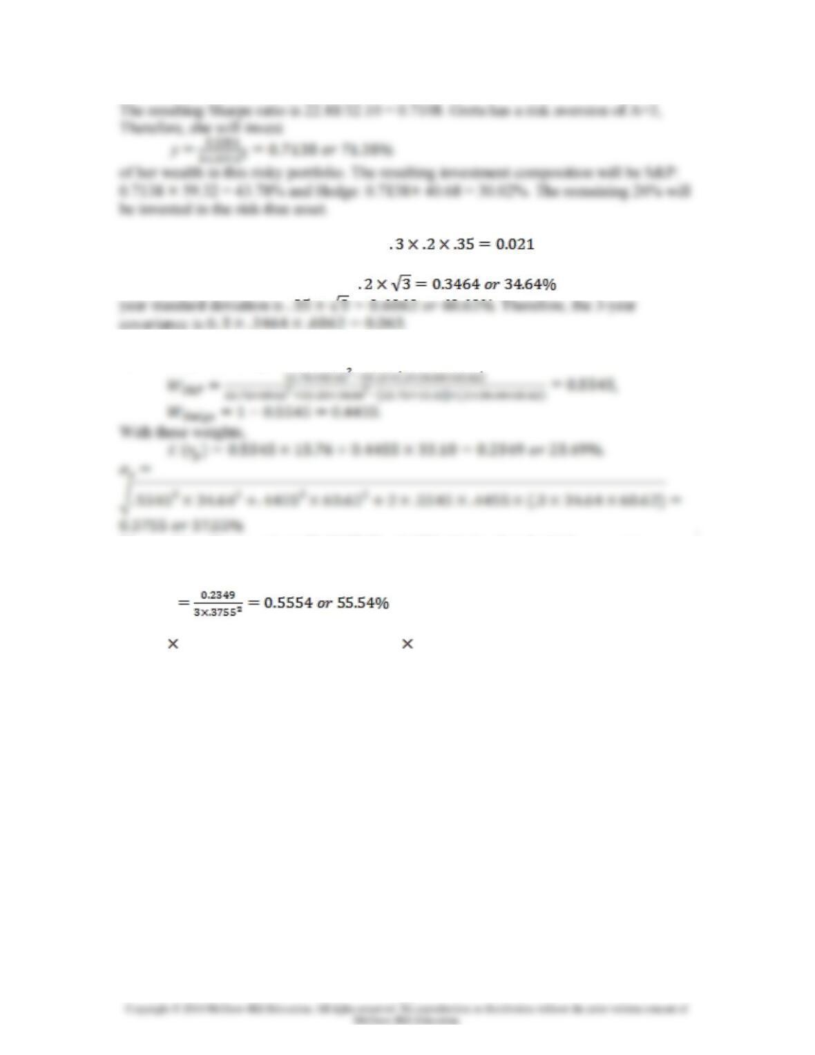
With these weights,
Chapter 7 – Optimal Risky Portfolios
7-9
24. With ρ = 0.3, the annual covariance is .
25. S&P 3-year standard deviation is . The hedge fund 3-
26. With a ρ=.3, the optimal asset allocation is
The resulting Sharpe ratio is 23.49/37.55 = 0.6256. Notice that the higher covariance
results in a poorer Sharpe ratio.
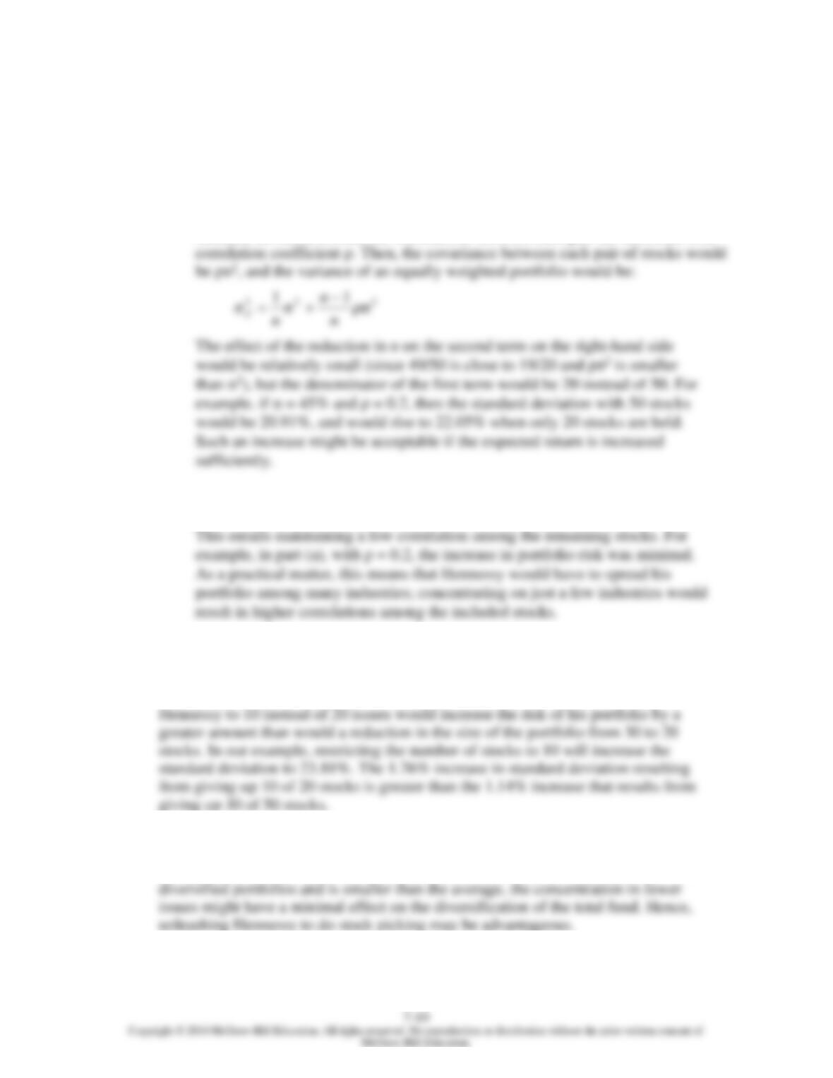
Greta will invest
y
of her wealth in this risky portfolio. The resulting investment composition will be S&P:
0.5554 55.45 =30.79% and hedge: 0.5554 44.55= 24.74%. The remaining 44.46%
will be invested in the risk-free asset.
Chapter 7 – Optimal Risky Portfolios
CFA PROBLEMS
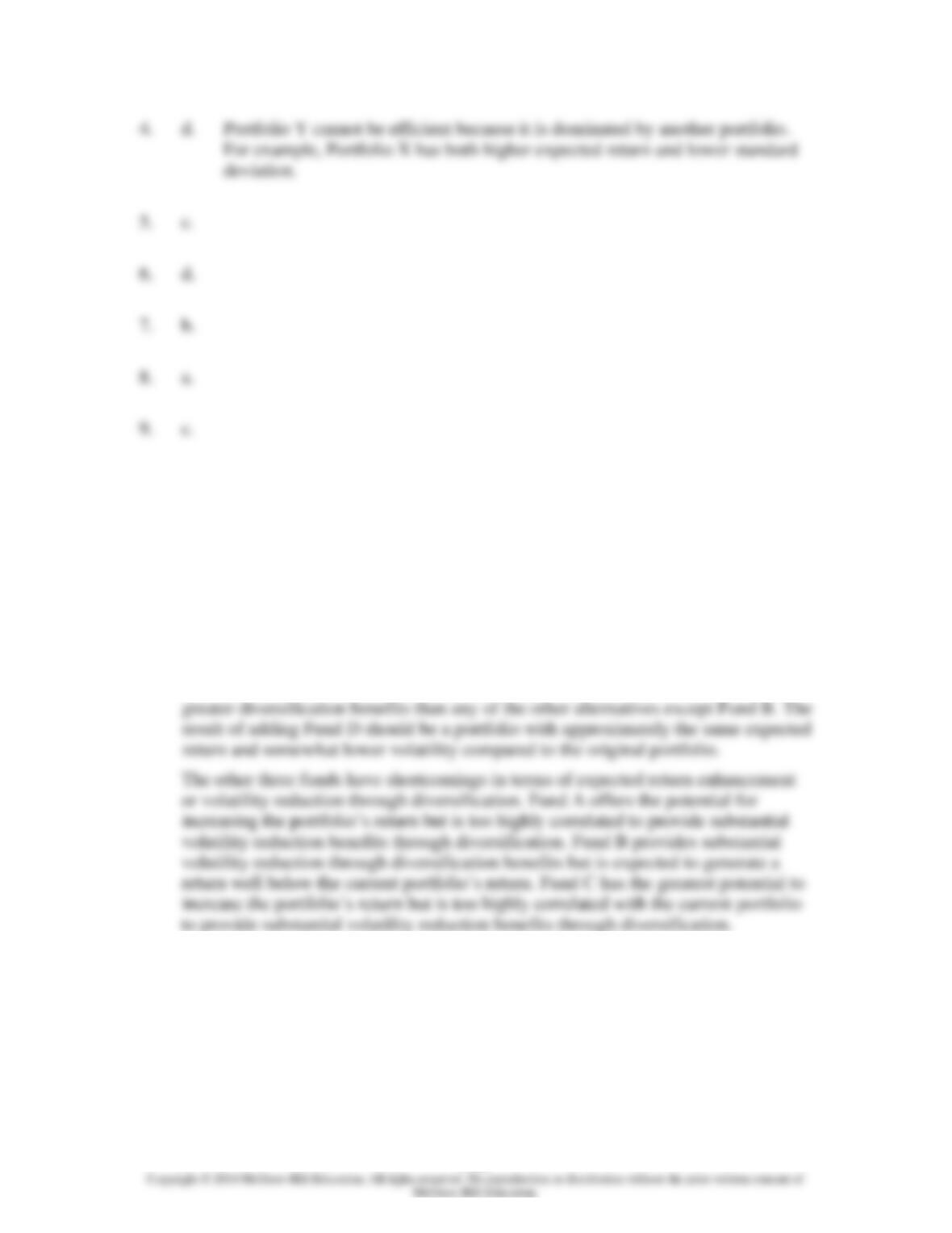
1. a. Restricting the portfolio to 20 stocks, rather than 40 to 50 stocks, will increase
the risk of the portfolio, but it is possible that the increase in risk will be
minimal. Suppose that, for instance, the 50 stocks in a universe have the same
standard deviation () and the correlations between each pair are identical, with
b. Hennessy could contain the increase in risk by making sure that he maintains
reasonable diversification among the 20 stocks that remain in his portfolio.
2. Risk reduction benefits from diversification are not a linear function of the number
of issues in the portfolio. Rather, the incremental benefits from additional
diversification are most important when you are least diversified. Restricting
3. The point is well taken because the committee should be concerned with the
volatility of the entire portfolio. Since Hennessy’s portfolio is only one of six well–
Chapter 7 – Optimal Risky Portfolios
7-11
10. Since we do not have any information about expected returns, we focus exclusively
on reducing variability. Stocks A and C have equal standard deviations, but the
correlation of Stock B with Stock C (0.10) is less than that of Stock A with Stock B
(0.90). Therefore, a portfolio composed of Stocks B and C will have lower total risk
than a portfolio composed of Stocks A and B.
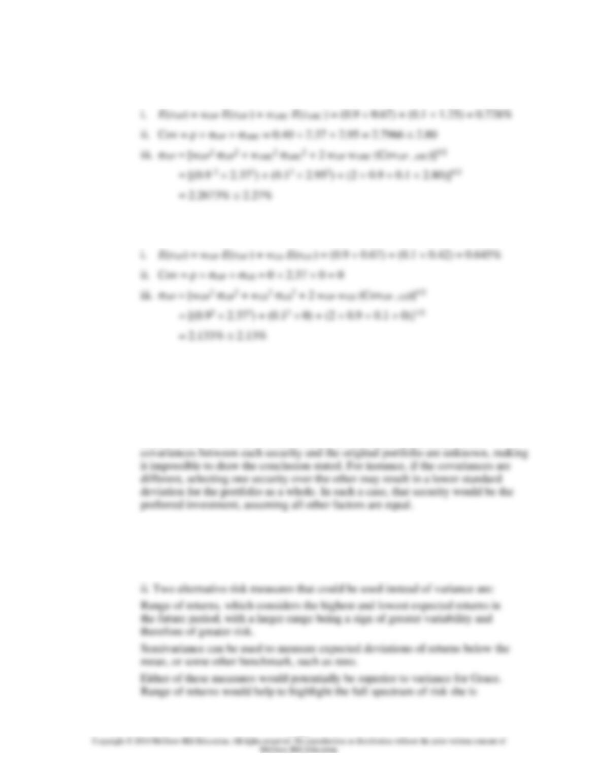
11. Fund D represents the single best addition to complement Stephenson’s current
portfolio, given his selection criteria. Fund D’s expected return (14.0 percent) has
the potential to increase the portfolio’s return somewhat. Fund D’s relatively low
correlation with his current portfolio (+0.65) indicates that Fund D will provide
Chapter 7 – Optimal Risky Portfolios
7-12
12. a. Subscript OP refers to the original portfolio, ABC to the new stock, and NP
to the new portfolio.
b. Subscript OP refers to the original portfolio, GS to government securities, and
NP to the new portfolio.
c. Adding the risk-free government securities would result in a lower beta for the
new portfolio. The new portfolio beta will be a weighted average of the
individual security betas in the portfolio; the presence of the risk-free securities
would lower that weighted average.
d. The comment is not correct. Although the respective standard deviations and
expected returns for the two securities under consideration are equal, the
e. i. Grace clearly expressed the sentiment that the risk of loss was more important
to her than the opportunity for return. Using variance (or standard deviation) as a
measure of risk in her case has a serious limitation because standard deviation
does not distinguish between positive and negative price movements.
Chapter 7 – Optimal Risky Portfolios
13. a. Systematic risk refers to fluctuations in asset prices caused by macroeconomic
factors that are common to all risky assets; hence systematic risk is often
b. Trudy should explain to the client that picking only the top five best ideas
would most likely result in the client holding a much more risky portfolio. The
total risk of a portfolio, or portfolio variance, is the combination of systematic
risk and firm-specific risk.
The systematic component depends on the sensitivity of the individual assets