Chapter 06 – Risk Aversion and Capital Allocation to Risky Assets
6-1
CHAPTER 6: RISK AVERSION AND
CAPITAL ALLOCATION TO RISKY ASSETS
PROBLEM SETS
2. (b) A higher borrowing is a consequence of the risk of the borrowers’ default. In perfect
markets with no additional cost of default, this increment would equal the value of the
3. Assuming no change in risk tolerance, that is, an unchanged risk aversion coefficient
(A), then higher perceived volatility increases the denominator of the equation for the
4. a. The expected cash flow is: (0.5 $70,000) + (0.5 200,000) = $135,000
With a risk premium of 8% over the risk-free rate of 6%, the required rate of return
b. If the portfolio is purchased for $118,421, and provides an expected cash inflow of
$135,000, then the expected rate of return [E(r)] is derived as follows:
c. If the risk premium over T-bills is now 12%, then the required return is:
6% + 12% = 18%
Chapter 06 – Risk Aversion and Capital Allocation to Risky Assets
6-2
5. When we specify utility by U = E(r) – 0.5A , the utility level for T-bills is: 0.07
6. Points on the curve are derived by solving for E(r) in the following equation:
The values of E(r), given the values of , are therefore:
2
E(r)
0.00
0.0000
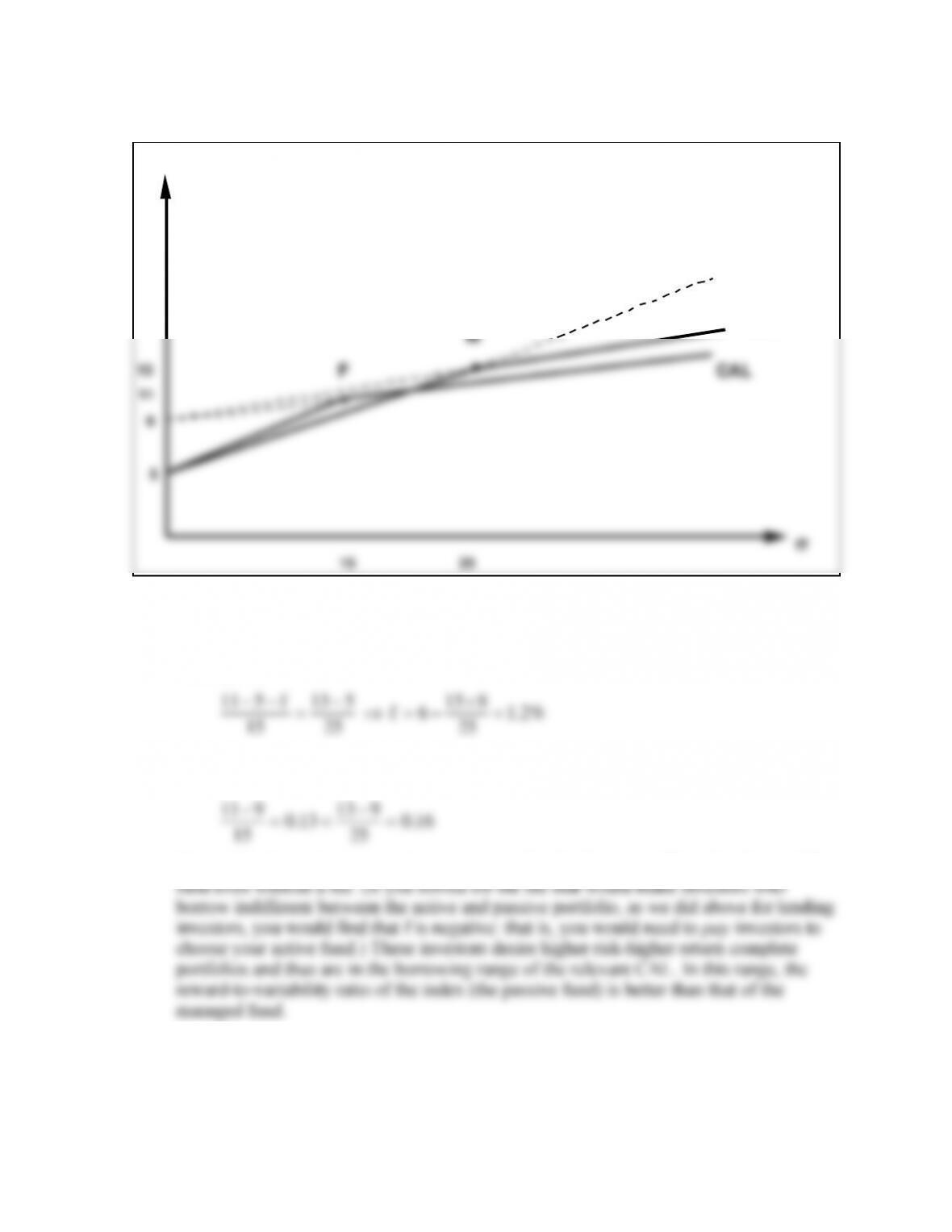
0.05000
0.05
0.0025
0.05375
0.10
0.0100
0.06500
0.15
0.0225
0.08375
0.20
0.0400
0.11000
0.25
0.0625
0.14375
Chapter 06 – Risk Aversion and Capital Allocation to Risky Assets
6-3
E(r)
5
4
U(Q6,A=3)
U(Q7,A=4)
U(Q8,A=0)
U(Q9,A<0)
7. Repeating the analysis in Problem 6, utility is now:
U = E(r) – 0.5A = E(r) – 2.0 = 0.04
The equal-utility combinations of expected return and standard deviation are presented
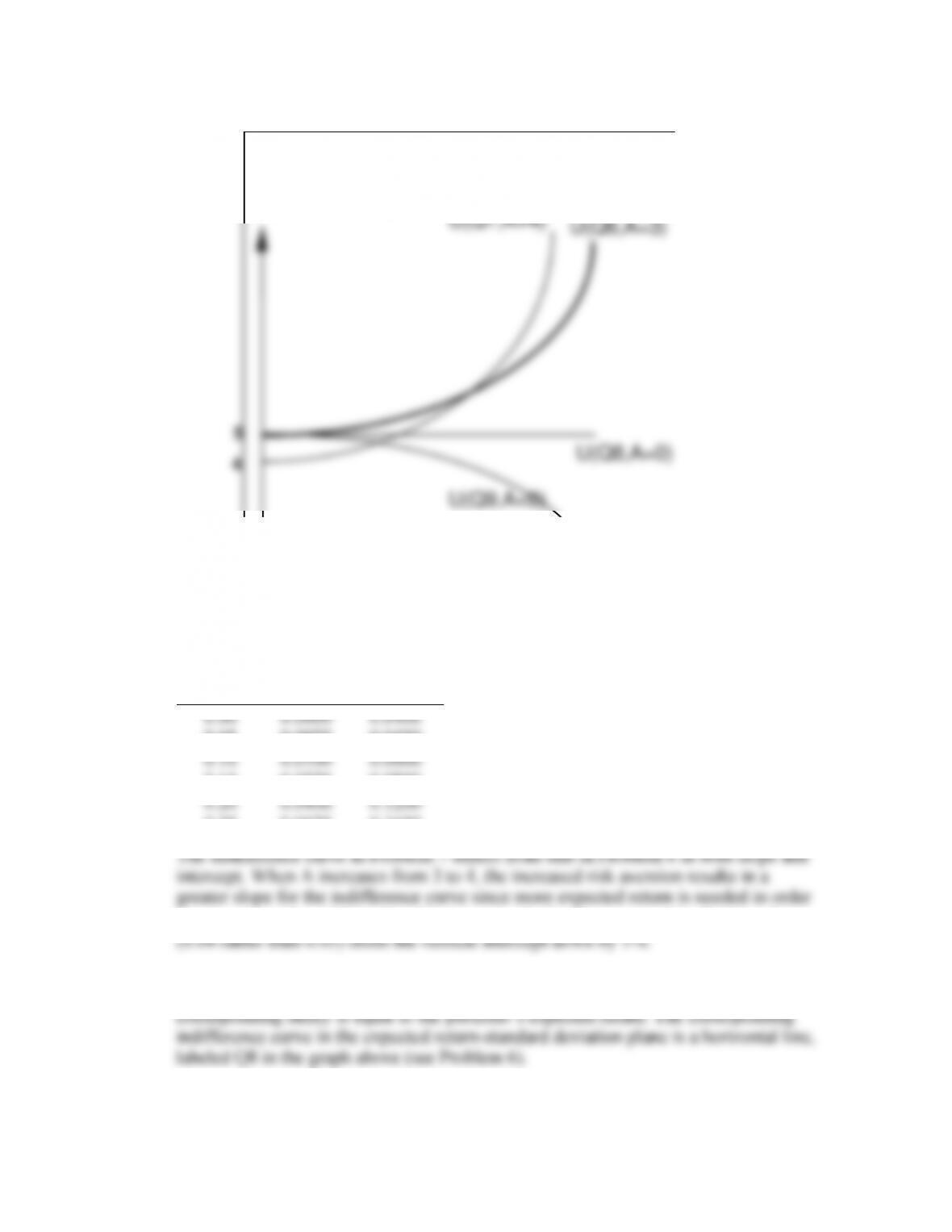
in the table below. The indifference curve is the upward sloping line in the graph above,
labeled Q7 (for Question 7).
2
E(r)
0.00
0.0000
0.0400
0.05
0.0025
0.0450
0.10
0.0100
0.0600
0.15
0.0225
0.0850
0.20
0.0400
0.1200
0.25
0.0625
0.1650
to compensate for additional . The lower level of utility assumed for Problem 7
8. The coefficient of risk aversion for a risk neutral investor is zero. Therefore, the
Chapter 06 – Risk Aversion and Capital Allocation to Risky Assets
9. A risk lover, rather than penalizing portfolio utility to account for risk, derives greater
utility as variance increases. This amounts to a negative coefficient of risk aversion. The
10. The portfolio expected return and variance are computed as follows:
(1)
WBills
(2)
rBills
(3)
WIndex
(4)
rIndex
rPortfolio
(1)(2)+(3)(4)
Portfolio
(3) 20%
2 Portfolio
0.0
5%
1.0
13.5%
13.5% = 0.135
20% = 0.20
0.0400
0.2
5%
0.8
13.5%
11.8% = 0.118
16% = 0.16
0.0256
0.4
5%
0.6
13.5%
10.1% = 0.101
12% = 0.12
0.0144
0.6
5%
0.4
13.5%
8.4% = 0.084
8% = 0.08
0.0064
0.8
5%
0.2
13.5%
6.7% = 0.067
4% = 0.04
0.0016
1.0
5%
0.0
13.5%
5.0% = 0.050
0% = 0.00
0.0000
11. Computing utility from U = E(r) – 0.5 A = E(r) – 1.5 , we arrive at the values in
the column labeled U(A = 3) in the following table:
WBills
WIndex
rPortfolio
Portfolio
2Portfolio
U(A = 3)
U(A = 5)
0.0
1.0
0.135
0.20
0.0400
0.0750
0.0350
0.2
0.8
0.118
0.16
0.0256
0.0796
0.0540
0.4
0.6
0.101
0.12
0.0144
0.0794
0.0650
0.6
0.4
0.084
0.08
0.0064
0.0744
0.0680
0.8
0.2
0.067
0.04
0.0016
0.0646
0.0630
1.0
0.0
0.050
0.00
0.0000
0.0500
0.0500
12. The column labeled U(A = 5) in the table above is computed from:
The more risk averse investors prefer the portfolio that is invested 40% in the market
13. Expected return = (0.7 18%) + (0.3 8%) = 15%
6-5
14.
Investment proportions:
30.0% in T-bills
0.7 25% =
17.5% in Stock A
0.7 32% =
22.4% in Stock B
0.7 43% =
30.1% in Stock C
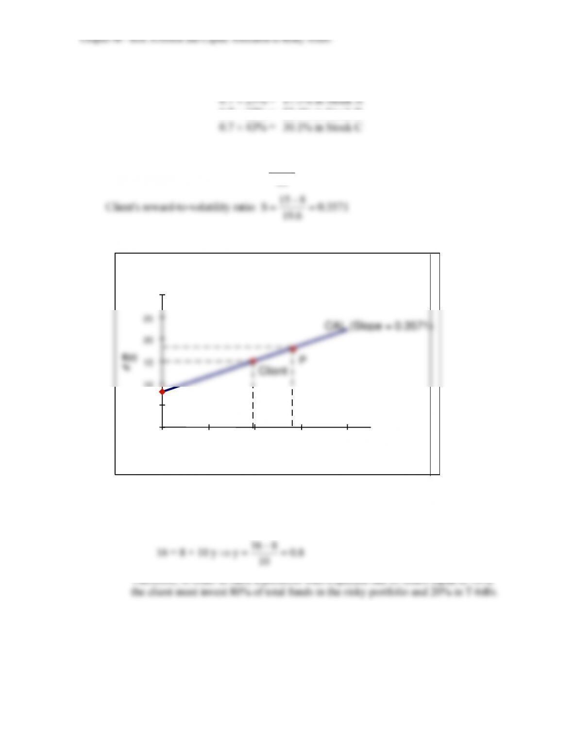
15. Your reward-to-volatility ratio:
3571.0
28
818
S=
−
=
3571.0
S=
=
6.19
815
−
16.
Client
P
0
5
10
15
20
25
30
0
10
20
30
40
()
E(r)
%
CAL (Slope = 0.3571)
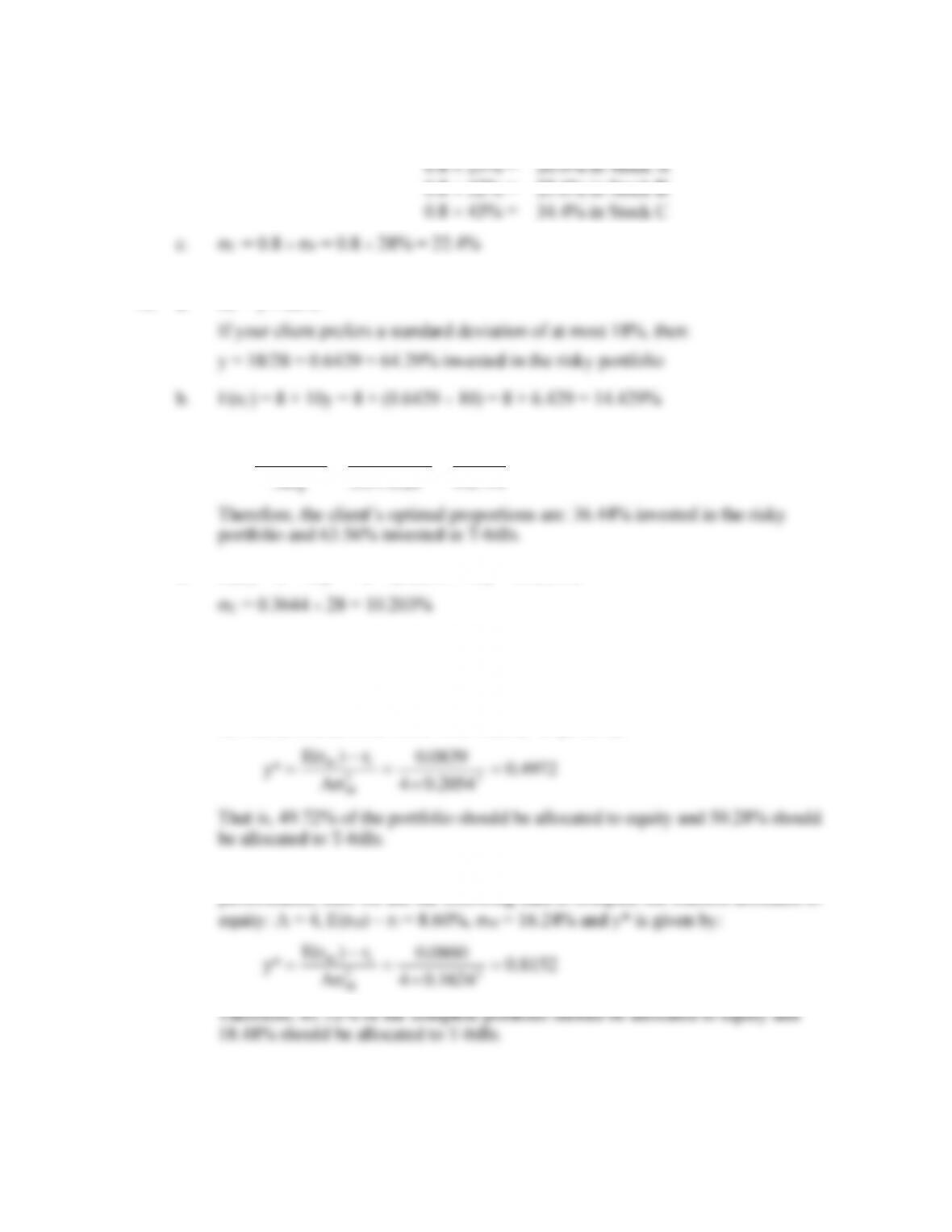
17. a. E(rC) = rf + y[E(rP) – rf] = 8 + y(18 − 8)
If the expected return for the portfolio is 16%, then:
816
−
Chapter 06 – Risk Aversion and Capital Allocation to Risky Assets
6-6
b.
Client’s investment proportions:
20.0% in T-bills
0.8 25% =
20.0% in Stock A
0.8 32% =
25.6% in Stock B
0.8 43% =
34.4% in Stock C
18. a. C = y 28%
19. a. y*
0.3644
0.2744
0.10
0.283.5
0.080.18
Aσ
r)E(r
22
P
fP ==
−
=
−
=
b. E(rC) = 8 + 10y* = 8 + (0.3644 10) = 11.644%
20. a. If the period 1926 – 2005 is assumed to be representative of future expected
performance, then we use the following data to compute the fraction allocated to
equity: A = 4, E(rM) − rf = 8.39%, M = 20.54% (we use the standard deviation of
the risk premium from Table 6.8). Then y* is given by:
0.4972
0.20544
0.0839
Aσ
r)E(r
y* 22
M
fM =
=
−
=
That is, 49.72% of the portfolio should be allocated to equity and 50.28% should
be allocated to T-bills.
b. If the period 1986 – 2005 is assumed to be representative of future expected
performance, then we use the following data to compute the fraction allocated to
0.8152
0.16244
0.0860
Aσ
r)E(r
y* 22
M
fM =
=
−
=
Chapter 06 – Risk Aversion and Capital Allocation to Risky Assets
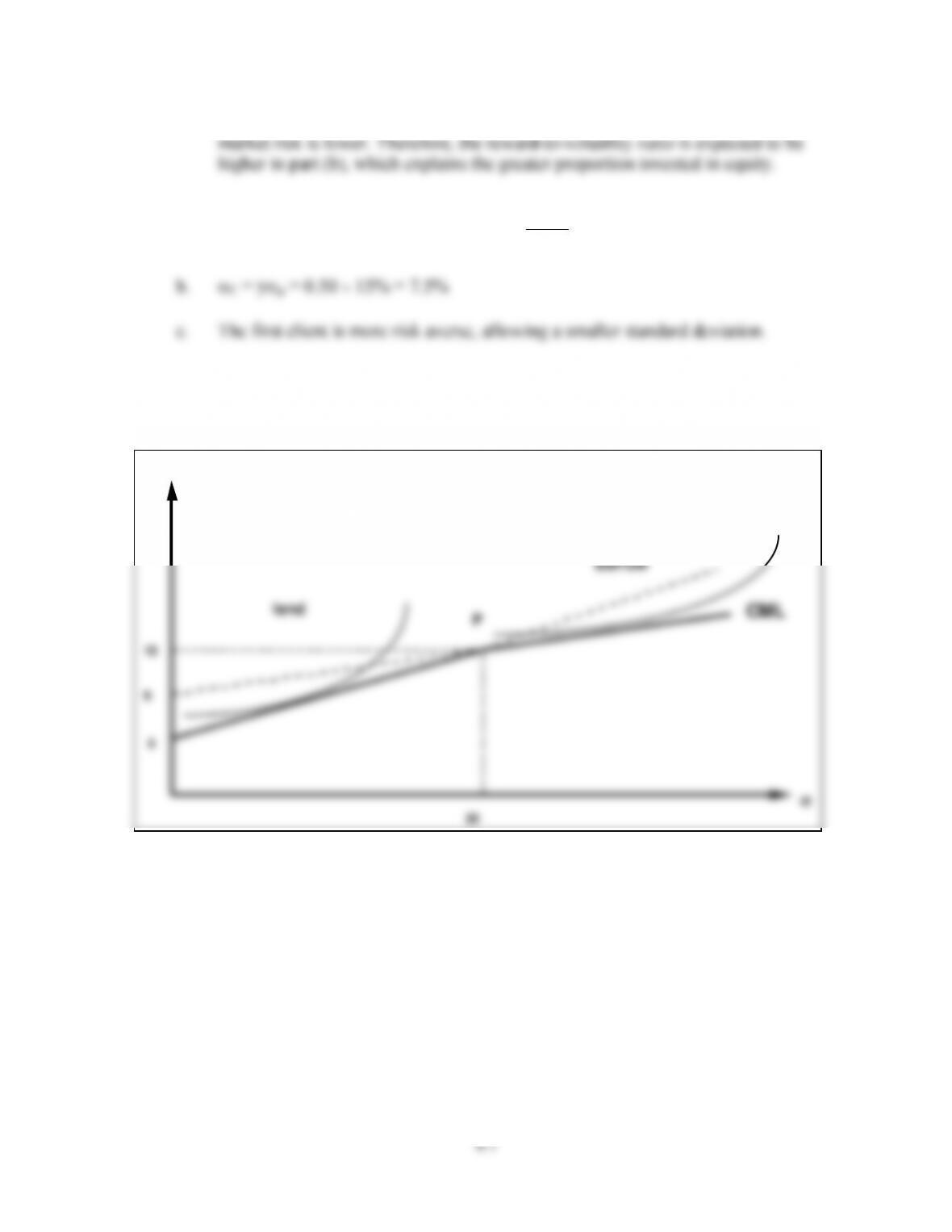
c. In part (b), the market risk premium is expected to be higher than in part (a) and
21. a. E(rC) = 8% = 5% + y(11% – 5%)
5.0
511
58
y=
−
−
=
22. Data: rf = 5%, E(rM) = 13%, M = 25%, and
B
f
r
= 9%
The CML and indifference curves are as follows:
P
borrow
lend CAL
E(r)
5
9
13
25
CML
0.15
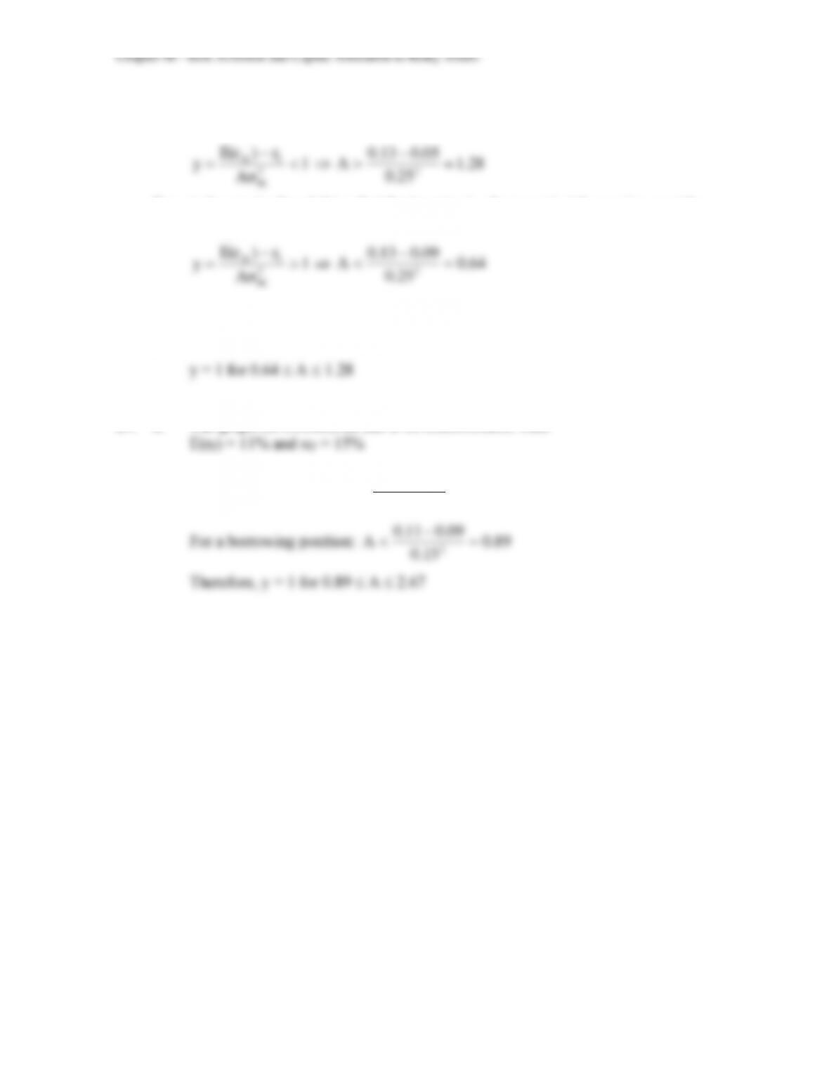
23. For y to be less than 1.0 (so that the investor is a lender), risk aversion (A) must be
large enough such that:
1
Aσ
r)E(r
y2
M
fM
−
=
1.28
0.25
0.050.13
A2=
−
For y to be greater than 1.0 (so that the investor is a borrower), risk aversion must be
small enough such that:
1
Aσ
r)E(r
y2
M
−
=
0.64
0.25
0.090.13
A2=
−
For values of risk aversion within this range, the client will neither borrow nor lend,
but instead will hold a complete portfolio comprised only of the optimal risky
portfolio:
24. a. The graph for Problem 22 has to be redrawn here, with:
b. For a lending position:
2.67
0.15
0.050.11
A2=
−
0.090.11
−
Chapter 06 – Risk Aversion and Capital Allocation to Risky Assets
6-9
MCML
E(r)
5
9
13
25
11
15
CALF
25. The maximum feasible fee, denoted f, depends on the reward-to-variability ratio.
For y < 1, the lending rate, 5%, is viewed as the relevant risk-free rate, and we solve for
f as follows:
25
513
15
f511 −
=
−−
%2.1
25
815
6f =
−=
For y > 1, the borrowing rate, 9%, is the relevant risk-free rate. Then we notice that,
even without a fee, the active fund is inferior to the passive fund because:
16.0
25
913
13.0
15
911 =
−
=
−
More risk tolerant investors (who are more inclined to borrow) will not be clients of the
Chapter 06 – Risk Aversion and Capital Allocation to Risky Assets
6-10
26. a. Slope of the CML
20.0
25
813 =
−
=
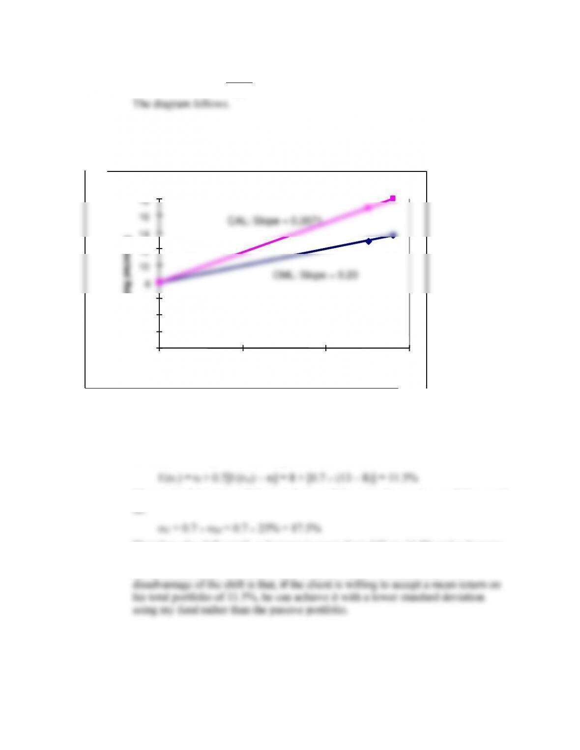
b. My fund allows an investor to achieve a higher mean for any given standard deviation than would
a passive strategy, i.e., a higher expected return for any given level of risk.
CML and CAL
0
2
4
6
8
10
12
14
16
18
0
10
20
30
Standard Deviation
Expected Retrun
CAL: Slope = 0.3571
CML: Slope = 0.20
27. a. With 70% of his money invested in my fund’s portfolio, the client’s expected
return is 15% per year and standard deviation is 19.6% per year. If he shifts that
money to the passive portfolio (which has an expected return of 13% and standard
deviation of 25%), his overall expected return becomes:
The standard deviation of the complete portfolio using the passive portfolio would
be:
Therefore, the shift entails a decrease in mean from 14% to 11.5% and a decrease
in standard deviation from 19.6% to 17.5%. Since both mean return and standard
deviation decrease, it is not yet clear whether the move is beneficial. The
Chapter 06 – Risk Aversion and Capital Allocation to Risky Assets
6-11
To achieve a target mean of 11.5%, we first write the mean of the complete
portfolio as a function of the proportion invested in my fund (y):
Our target is: E(rC) = 11.5%. Therefore, the proportion that must be invested in my
fund is determined as follows:
10
85.11
−
The standard deviation of this portfolio would be:
Thus, by using my portfolio, the same 11.5% expected return can be achieved with
b. The fee would reduce the reward-to-volatility ratio, i.e., the slope of the CAL. The
client will be indifferent between my fund and the passive portfolio if the slope of
the after-fee CAL and the CML are equal. Let f denote the fee:
f10
f818 −
−−
25
Setting these slopes equal we have:
20.0
28
f10 =
−
10 − f = 28 0.20 = 5.6 f = 10 − 5.6 = 4.4% per year
28. a. The formula for the optimal proportion to invest in the passive portfolio is:
2
M
fM
Aσ
r)E(r
y* −
=
Substitute the following: E(rM) = 13%; rf = 8%; M = 25%; A = 3.5:
0.2286
0.253.5
0.080.13
y* 2=
−
=
b. The answer here is the same as the answer to Problem 27(b). The fee that you can
Chapter 06 – Risk Aversion and Capital Allocation to Risky Assets
CFA PROBLEMS
1. Utility for each investment = E(r) – 0.5 4
We choose the investment with the highest utility value.
Investment
Expected
return
E(r)
Standard
deviation
Utility
U
1
0.12
0.30
-0.0600
2
0.15
0.50
-0.3500
3
0.21
0.16
0.1588
4
0.24
0.21
0.1518
4. Indifference curve 2
8. Expected return for equity fund = T-bill rate + risk premium = 6% + 10% = 16%
10 =
Chapter 06 – Risk Aversion and Capital Allocation to Risky Assets
6-13
CHAPTER 6: APPENDIX
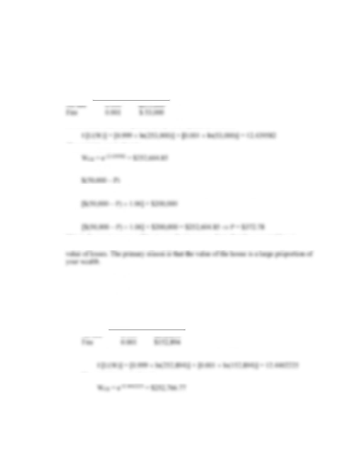
1. By year end, the $50,000 investment will grow to: $50,000 1.06 = $53,000
Without insurance, the probability distribution of end-of-year wealth is:
Probability
Wealth
No fire
0.999
$253,000
Fire
0.001
$ 53,000
For this distribution, expected utility is computed as follows:
The certainty equivalent is:
With fire insurance, at a cost of $P, the investment in the risk-free asset is:
Year-end wealth will be certain (since you are fully insured) and equal to:
Solve for P in the following equation:
This is the most you are willing to pay for insurance. Note that the expected loss is
“only” $200, so you are willing to pay a substantial risk premium over the expected
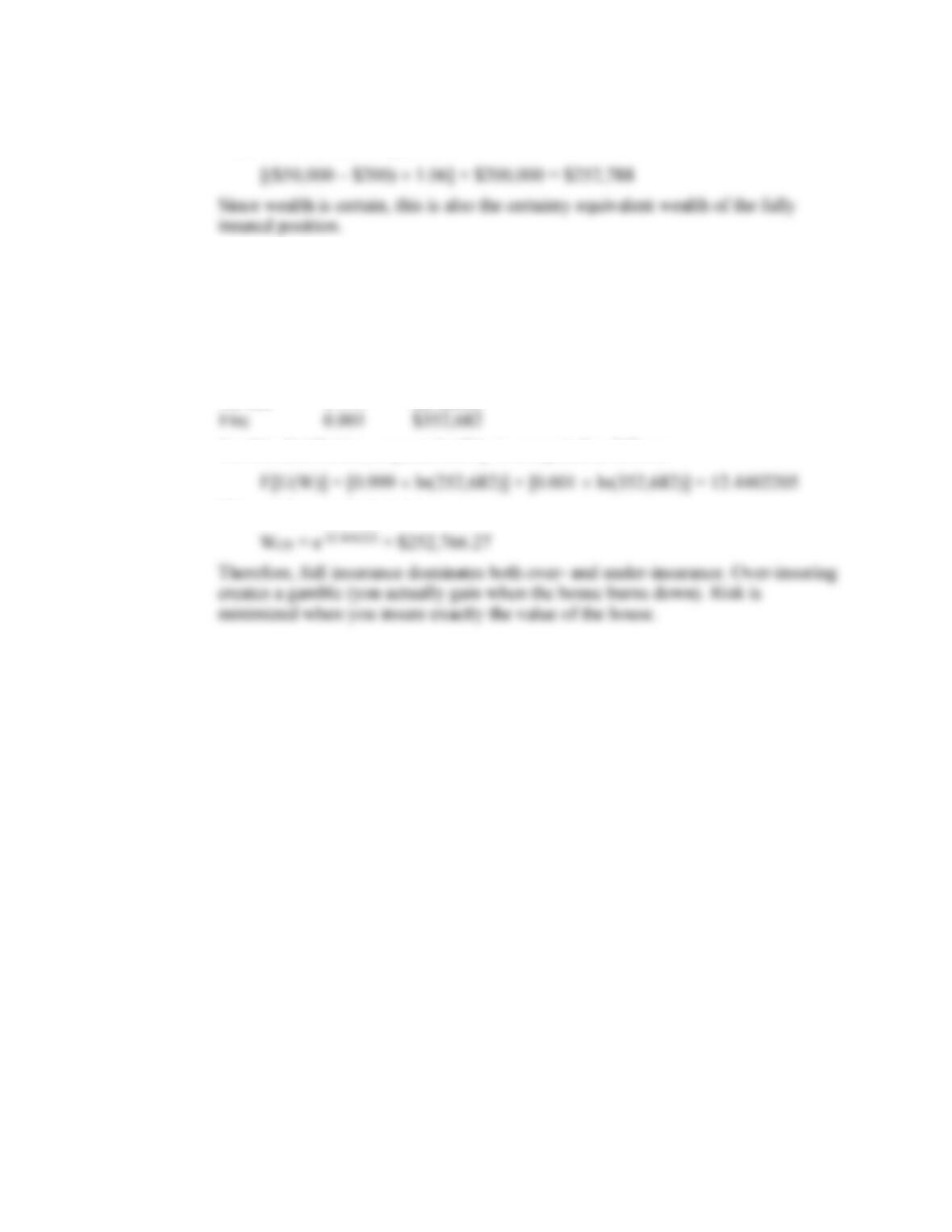
2. a. With insurance coverage for one-half the value of the house, the premium is
$100, and the investment in the safe asset is $49,900. By year end, the
investment of $49,900 will grow to: $49,900 1.06 = $52,894
If there is a fire, your insurance proceeds will be $100,000, and the probability
distribution of end-of-year wealth is:
Probability
Wealth
No fire
0.999
$252,894
Fire
0.001
$152,894
For this distribution, expected utility is computed as follows:
The certainty equivalent is:
Chapter 06 – Risk Aversion and Capital Allocation to Risky Assets
6-14
b. With insurance coverage for the full value of the house, costing $200, end-of-year
wealth is certain, and equal to:
c. With insurance coverage for 1½ times the value of the house, the premium is
$300, and the insurance pays off $300,000 in the event of a fire. The investment
in the safe asset is $49,700. By year end, the investment of $49,700 will grow
to: $49,700 1.06 = $52,682
The probability distribution of end-of-year wealth is:
Probability
Wealth
No fire
0.999
$252,682
Fire
0.001
$352,682
For this distribution, expected utility is computed as follows:
The certainty equivalent is: