Chapter 06 – Efficient Diversification
CHAPTER SIX
EFFICIENT DIVERSIFICATION
CHAPTER OVERVIEW
In this chapter, the concept of portfolio formation moves beyond the risky and risk-free asset
combinations of the previous chapter to include combinations of two or more risky assets. The
concept of risk reduction via diversification, created by combining securities with different
return patterns, is introduced. The student is introduced to analytical tools that are used to create
the lowest-risk portfolio that meets a target expected return. After finding the best diversified
combinations, the risk free asset is combined with the risky portfolio. The capital allocation line,
that is tangent to the so called efficient frontier of best diversified portfolios, will dominate all
risky portfolios regardless of the level of risk aversion.
LEARNING OBJECTIVES
Students should be able to calculate the standard deviation and return for two security portfolios
find the minimum variance combinations of two securities. Upon completion of this chapter the
student should have a full understanding of systematic and firm-specific risk, and of how the
portfolio’s firm-specific risk can be reduced by combining securities with differing patterns of
returns. The student should be able to quantify this concept by being able to calculate and
interpret covariance and correlation coefficients.
Chapter 06 – Efficient Diversification
CHAPTER OUTLINE
1. Diversification and Portfolio Risk
2. Asset Allocation with Two Risky Assets
PPT 6-2 through PPT 6-17
When we put stocks in a portfolio, p < (Wii). When Stock 1 has a return > E[r1], it is likely
that Stock 2 has a return < E[r2] so that return on the portfolio that contains stocks 1 and 2
remains close to its expected return. Covariance and correlation measure the tendency for r1 to
be above expected when r2 is below expected.
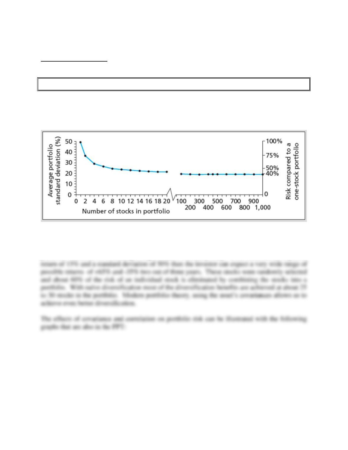
Text Figure 6.2
Text Figure 6.2 illustrates how adding securities to the portfolio reduces the portfolio risk as
measured by the standard deviation. Notice size of the standard deviation of a single stock
portfolio. At about 50%, holding a single stock is extremely risky. If the stock has an expected
Chapter 06 – Efficient Diversification
Chapter 06 – Efficient Diversification
Return and Risk of a Two Asset Portfolio
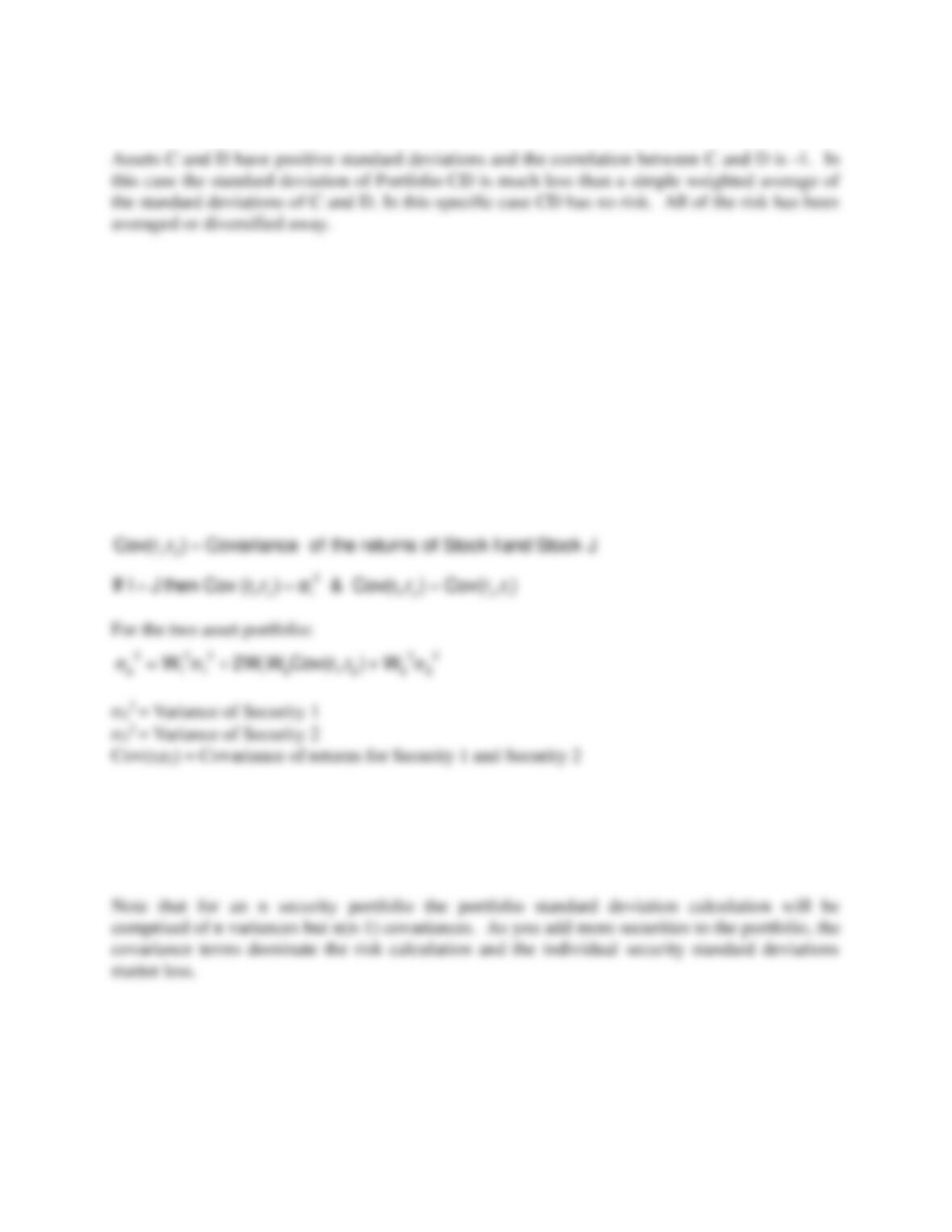
The expected return of a portfolio is simply a weighted average of the returns of the portfolio
components. Because of the diversification effects however, the standard deviation of the
portfolio is not a simple weighted average of standard deviations of the components. The
relevant formulas are as follows:
The PPT provides ample detail about the correlation coefficient and about why correlations are
easier to interpret than covariance. This detail can be skipped if your students are reasonably
proficient in statistics.
portfolio the in securities # n ;rW)rE(
n
1i
i
i
p==
=
Wi
i=1
n= 1Wi
i=1
nWi
Wi
i=1i=1
n= 1
= =
=n
1I
n
1J JIJI
2
p)]r,Cov(r W[Wσ
portfolio the in stocks of number total The n
lyrespective J and I stock in invested portfolio total the of PercentageW,W JI
=
=
Ch 6-22
E(r)
13%
12% 20% St. Dev
TWO-SECURITY PORTFOLIOS WITH
DIFFERENT CORRELATIONS
Stock A Stock B
WA= 0%
WB= 100%
r= -1
→
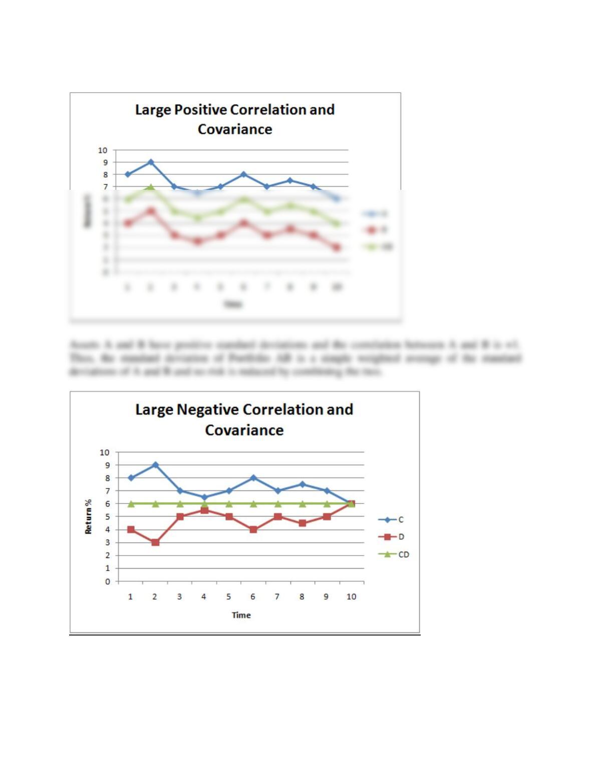
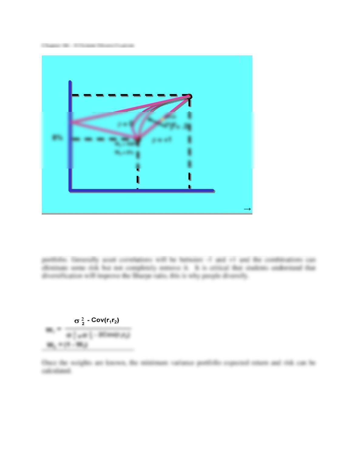
The graph depicts return/risk combinations of two securities, A and B for different hypothetical
correlation coefficients. If there is a perfect positive correlation between A and B, combining
the two securities yields no diversification benefits and combinations of A and B fall on a
straight line because in this case p = Wii. However if the assets are perfectly negatively
correlated, we can combine the two securities to completely eliminate variance in the combined
In the two-asset case it is fairly easy to calculate the minimum variance weight with the
following equations:
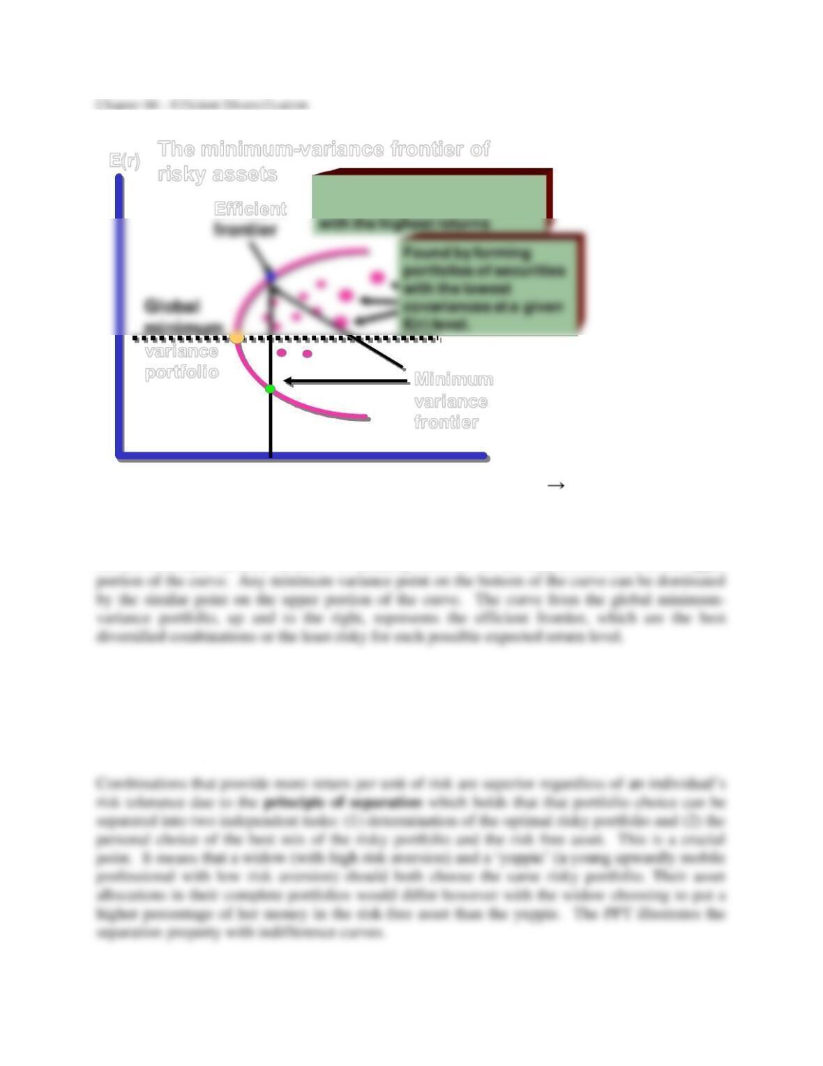
E(r) The minimum-variance frontier of
risky assets
variance
portfolio
Efficient
Minimum
variance
frontier
St. Dev.
Efficient Frontier is the best
diversified set of investments
→
From this point in the development it is an easy step to illustrate the minimum variance set and
the efficient frontier for large numbers of securities. Considering many risky asset combinations
(and always keeping the combinations that have the least risk for a given return level) one can
build a minimum-variance frontier. In actuality however we are only concerned with the upper
The text also illustrates the benefits of diversification, using historical data to examine the effects
of including stocks and bonds in a portfolio during some of extreme loss years. The overall
standard deviation of the diversified portfolio that includes bonds is smaller than the standard
deviation of either stocks or bonds individually. Thus, combinations that include bonds are
likely to have higher Sharpe ratios, that is, more return per unit of risk.
3. The Optimal Risky Portfolio with a Risk-Free Asset
4. Efficient Diversification with Many Risky Assets
PPT 6-18 through PPT 6-29
The inclusion of a risk-free asset in a portfolio results in a single combination of stock and bonds
that is optimal when that portfolio is combined with the risk-free asset. As explained in Chapter
5 the resulting capital allocation line is now linear. This is because the covariance between the
risk free asset and the risky portfolio is zero.
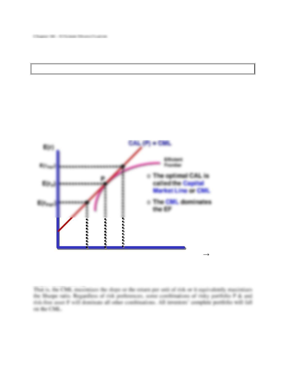
At this point the Capital Market Line or CML can be developed as the optimal Capital Asset
Line (CAL) that results from combining the risk free asset with the efficient frontier as depicted
below:
The Capital Market Line or CML
F
Risk Free
P&F →
PP&F
CAL(P) = Capital Market Line or CML dominates other lines because it has the largest slope or
equivalently, the largest Sharpe ratio
Slope = (E(rp) – rf) / p
E(r)
The Capital Market Line or CML
P
F
Risk Free
P&F →
Efficient
Frontier
PP&F
E(rP&F)
CML
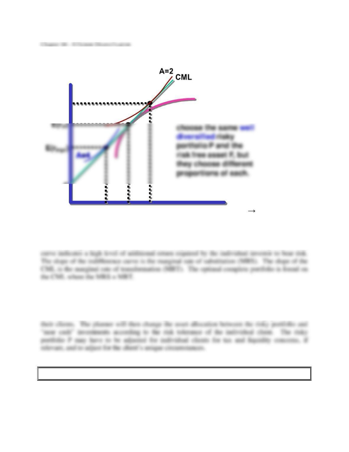
A=2
Both investors
In this graph we have two investors with different levels of risk aversion. The A coefficient of 2
indicates a high level of risk aversion and a steeper indifference curve. A steep indifference
Practical Implications
The analyst or planner should identify what they believe will be the best performing well–
diversified portfolio, call it “P”. P may include funds, stocks, and bonds, as well as international
and other alternative investments. This portfolio will serve as the starting point for all
5. A Single Index Asset Market
PPT 6-30 through PPT 6-38
We have learned that investors should diversify, thus individual securities will be held in a
portfolio.
Chapter 06 – Efficient Diversification
The risk that cannot be diversified away, i.e., the risk that remains when the stock is put into a
portfolio, is called systematic risk. Systematic risk is also called non-diversifiable risk.
Systematic risk arises from events that affect the entire economy. Examples of such events
include a change in interest rates or GDP; or a financial crisis such as that which occurred in
The single-factor model of excess returns can be used to estimate a security’s beta.
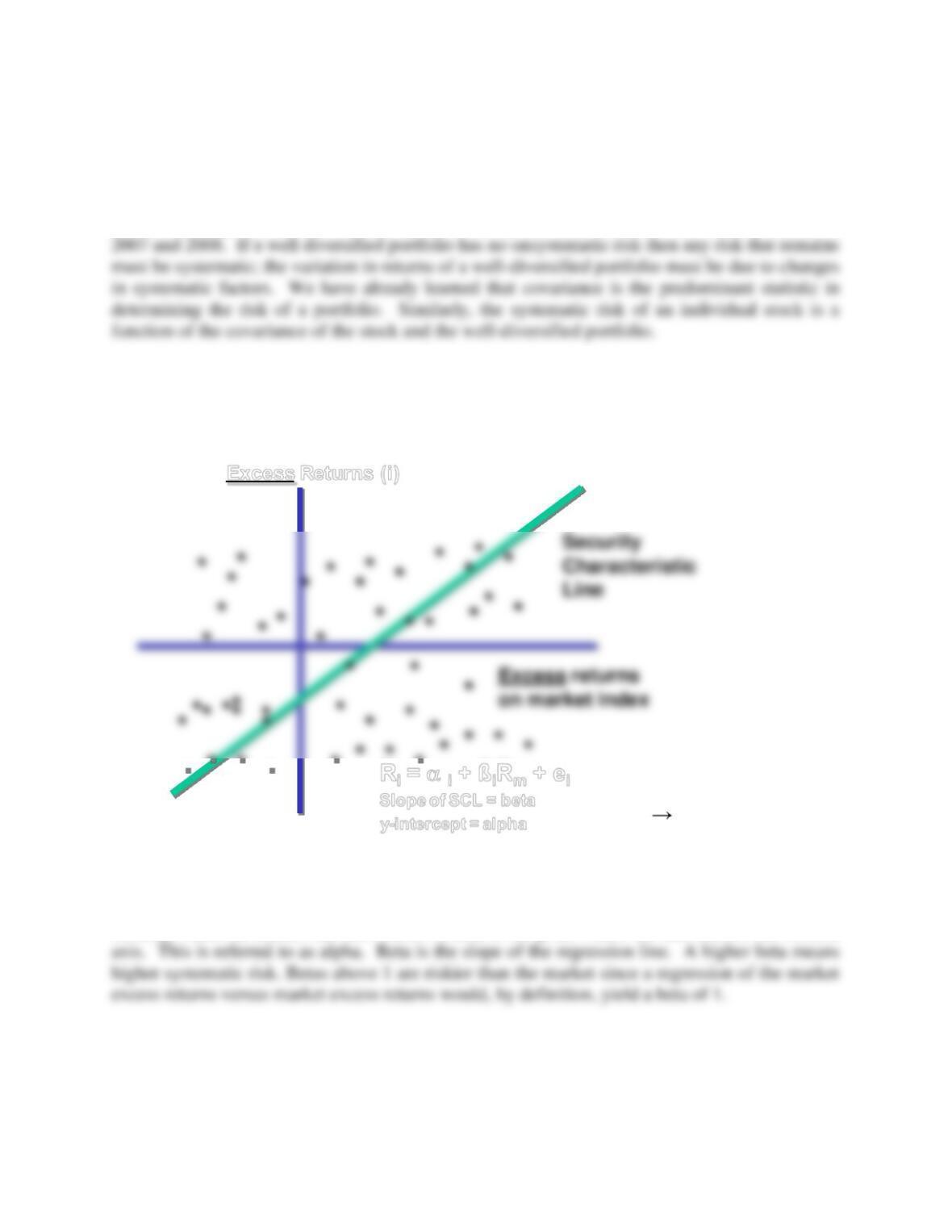
Estimating the Index Model
Excess Returns (i)
. . .
. .
. .
Ri= ai+ ßiRm+ ei
Slope of SCL = beta
y-intercept = alpha →
Scatter
Plot
Each point would represent a sample pair of excess returns observed for a particular holding
period. A regression analysis will find the “best fit” line for the data. The expected return for the
security, when the market has zero excess return, is the point where the line crosses the vertical
Chapter 06 – Efficient Diversification
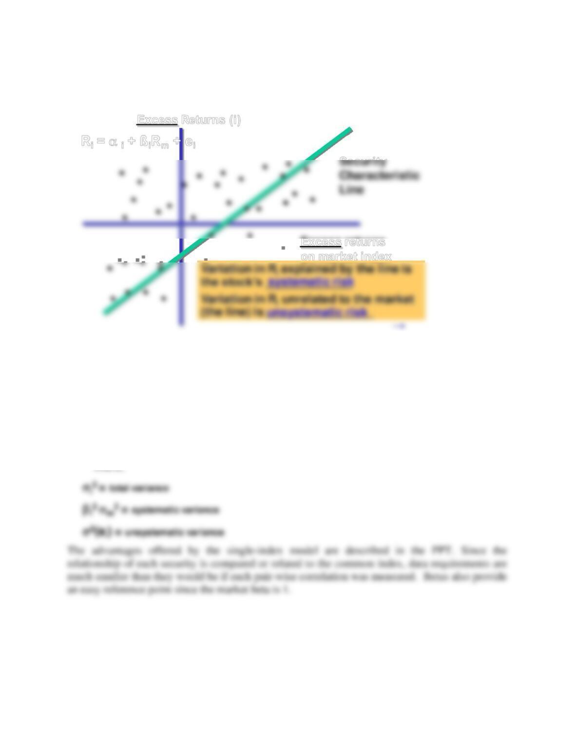
Estimating the Index Model
Excess Returns (i)
. ..
..
.
on market index
Scatter
Plot
Ri= ai+ ßiRm+ ei
The scatter plot can also be used to illustrate systematic and unsystematic risk. The risk is
related to the systematic or macroeconomic factor, in this case the market index. A stock’s total
risk, as measured by its standard deviation, can be partitioned into systematic and unsystematic
risk.
Measuring Components of Risk
i2 =
where;
bi2m2 + 2(ei)
Chapter 06 – Efficient Diversification
The Treynor-Black Model (advanced topic)
If a manager has the ability to find undervalued stocks, what strategy should a portfolio manager
use in investing in those stocks? The percentage of funds allocated to undervalued stocks
depends, in part, on the ability of the manager. If a manager has perfect foresight, theoretically
all funds should be placed in the most undervalued stocks. If the manager has substantial funds,
The Treynor-Black Model is used to combine an actively-managed portfolio with a passively-
managed portfolio. A reward-to-variability measure, similar to the Sharpe measure, is used to
determine optimal allocations in the active and passive portfolio. To determine optimal
By combining the active and passive portfolios, the manager can achieve a superior reward-to–
risk combination. Understanding the results of the Treynor-Black Model is best accomplished
through a graphical presentation. A graph is provided in the PPT. The standard Capital Market
The Treynor-Black Model details (advanced topic)
“Well performing” individual stocks held in diversified portfolios can be evaluated by the
stock’s alpha in relation to the stock’s unsystematic risk. Suppose an investor holds a passive
portfolio M but believes that an individual security has a positive alpha. A positive alpha implies
the security is undervalued. Suppose Google has the positive alpha. Adding Google moves the
overall portfolio away from the diversified optimum, thus bearing residual risk that could be
eliminated; however, it might be worth it to earn the positive alpha. We need to determine the
Chapter 06 – Efficient Diversification
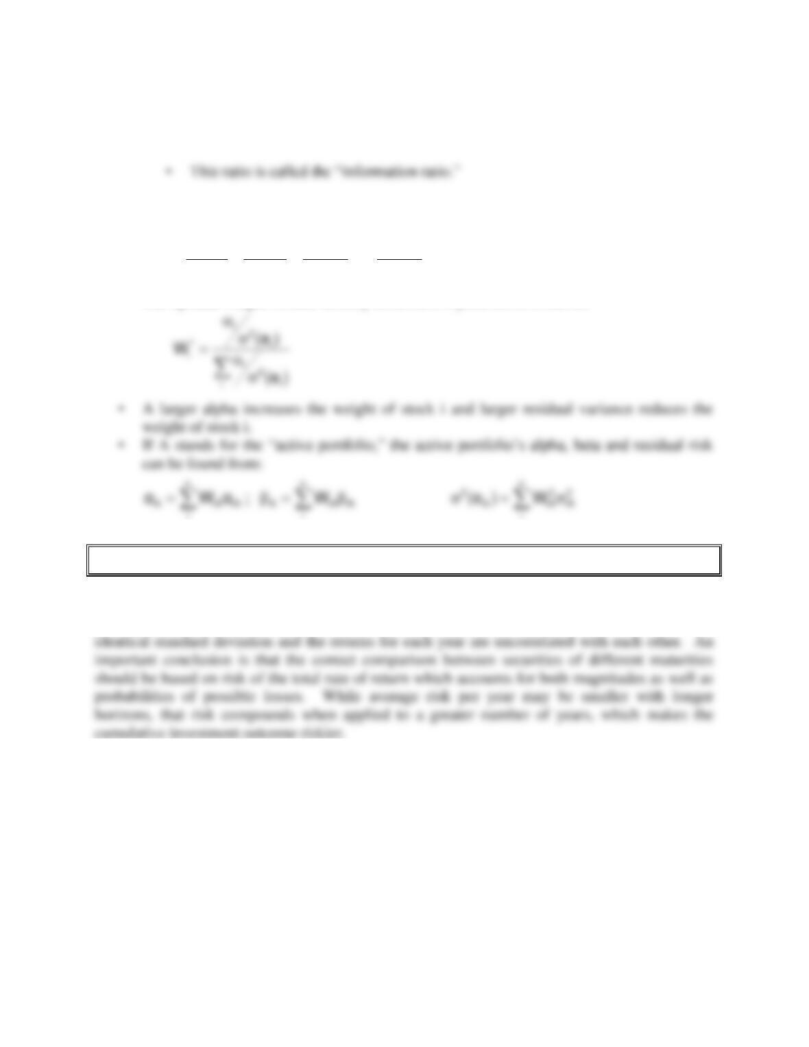
• For multiple stocks in the active portfolio:
• The optimal weight of each security in the active portfolio is found as:
6. Risk of Long-Term Investments
PPT 6-39 through PPT 6-40
The last section of this chapter provides a comparison of the variance and standard deviation of
short-term and long-term investments. PPT 6-41 and PPT 6-42 present a calculation for variance
and standard deviation on an investment. The investment’s rate of return in each year has an
)e(
...
)e()e()e( n
2
n
2
2
2
1
2
1
n
ii
2
i
a
+
a
+
a
=
a

Chapter 06 – Efficient Diversification
Excel Applications
Several Excel applications are discussed in the text and one Excel model is available on the
website that can be used to apply the concepts covered in Chapter 6. The model constructs an
efficient portfolio for many securities. The model constructs efficient combinations of the