Investments & Securities Chapter 6 A higher borrowing rate is a consequence of the risk

Chapter 6 – Capital Allocation to Risky Assets

6-

1

CHAPTER 6: CAPITAL ALLOCATION TO RISKY ASSETS

PROBLEM SETS

1. (e) The first two answer choices are incorrect because a highly risk averse investor

would avoid portfolios with higher risk premiums and higher standard deviations.

2. (b) A higher borrowing rate is a consequence of the risk of the borrowers’ default.

In perfect markets with no additional cost of default, this increment would equal the

3. Assuming no change in risk tolerance, that is, an unchanged risk-aversion

4. a. The expected cash flow is: (0.5 × $70,000) + (0.5 × 200,000) = $135,000.

With a risk premium of 8% over the risk-free rate of 6%, the required rate of

return is 14%. Therefore, the present value of the portfolio is:

$135,000/1.14 = $118,421

b. If the portfolio is purchased for $118,421 and provides an expected cash

c. If the risk premium over T-bills is now 12%, then the required return is:

6% + 12% = 18%

Chapter 6 – Capital Allocation to Risky Assets

6-

2

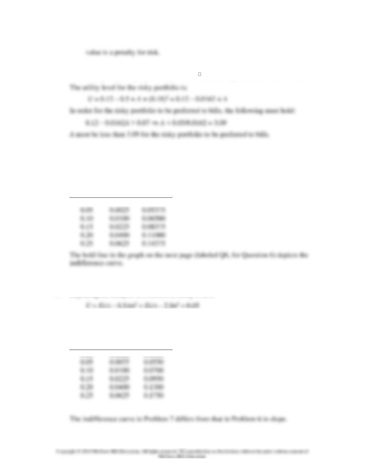
5. When we specify utility by U = E(r) – 0.5Aσ2, the utility level for T-bills is: 0.07

6. Points on the curve are derived by solving for E(r) in the following equation:

U = 0.05 = E(r) – 0.5Aσ2 = E(r) – 1.5σ2

The values of E(r), given the values of σ2, are therefore:



 2

E(r)

0.00

0.0000

0.05000

0.05

0.0025

0.05375

0.10

0.0100

0.06500

0.15

0.0225

0.08375

0.20

0.0400

0.11000

0.25

0.0625

0.14375

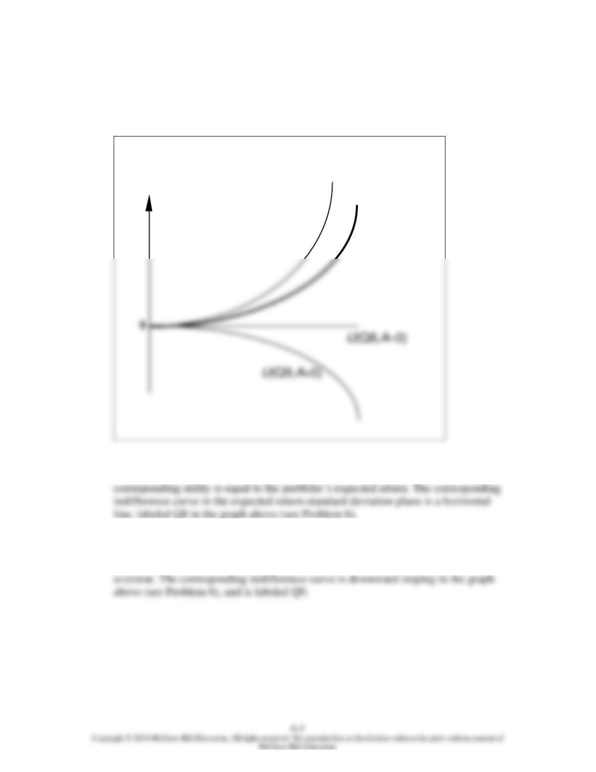
7. Repeating the analysis in Problem 6, utility is now:

The equal-utility combinations of expected return and standard deviation are

presented in the table below. The indifference curve is the upward sloping line in

the graph on the next page, labeled Q7 (for Question 7).



 2

E(r)

0.00

0.0000

Chapter 6 – Capital Allocation to Risky Assets

When A increases from 3 to 4, the increased risk aversion results in a greater

slope for the indifference curve since more expected return is needed in order to

compensate for additional σ.

E(r)

U(Q6,A=3)

U(Q7,A=4)

8. The coefficient of risk aversion for a risk neutral investor is zero. Therefore, the

9. A risk lover, rather than penalizing portfolio utility to account for risk, derives

greater utility as variance increases. This amounts to a negative coefficient of risk

Chapter 6 – Capital Allocation to Risky Assets

6-

4

10. The portfolio expected return and variance are computed as follows:

(1)

WBills

(2)

rBills

(3)

WIndex

(4)

rIndex

rPortfolio

(1)×(2)+(3)×(4)

Portfolio

(3) × 20%

 2 Portfolio

0.0

5%

1.0

13.0%

13.0% = 0.130

20% = 0.20

0.0400

0.0256

0.0064

0.0016

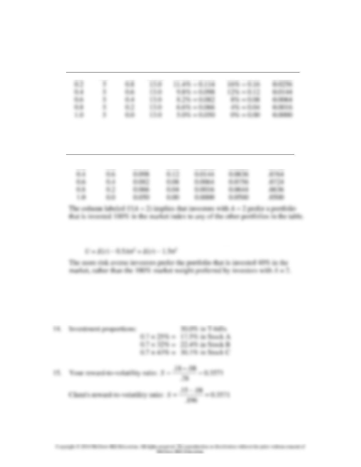
11. Computing utility from U = E(r) – 0.5 × Aσ2 = E(r) – σ2, we arrive at the values in

the column labeled U(A = 2) in the following table:

WBills

WIndex

rPortfolio

Portfolio

2Portfolio

U(A = 2)

U(A = 3)

0.0

1.0

0.130

0.20

0.0400

0.0900

.0700

0.2

0.8

0.114

0.16

0.0256

0.0884

.0756

0.6

0.4

0.082

0.08

0.0064

0.0756

.0724

0.8

0.2

0.066

0.04

0.0016

0.0644

.0636

12. The column labeled U(A = 3) in the table above is computed from:

13. Expected return = (0.7 × 18%) + (0.3 × 8%) = 15%

Standard deviation = 0.7 × 28% = 19.6%

Chapter 6 – Capital Allocation to Risky Assets

6-

5

16.

15

20

25

30

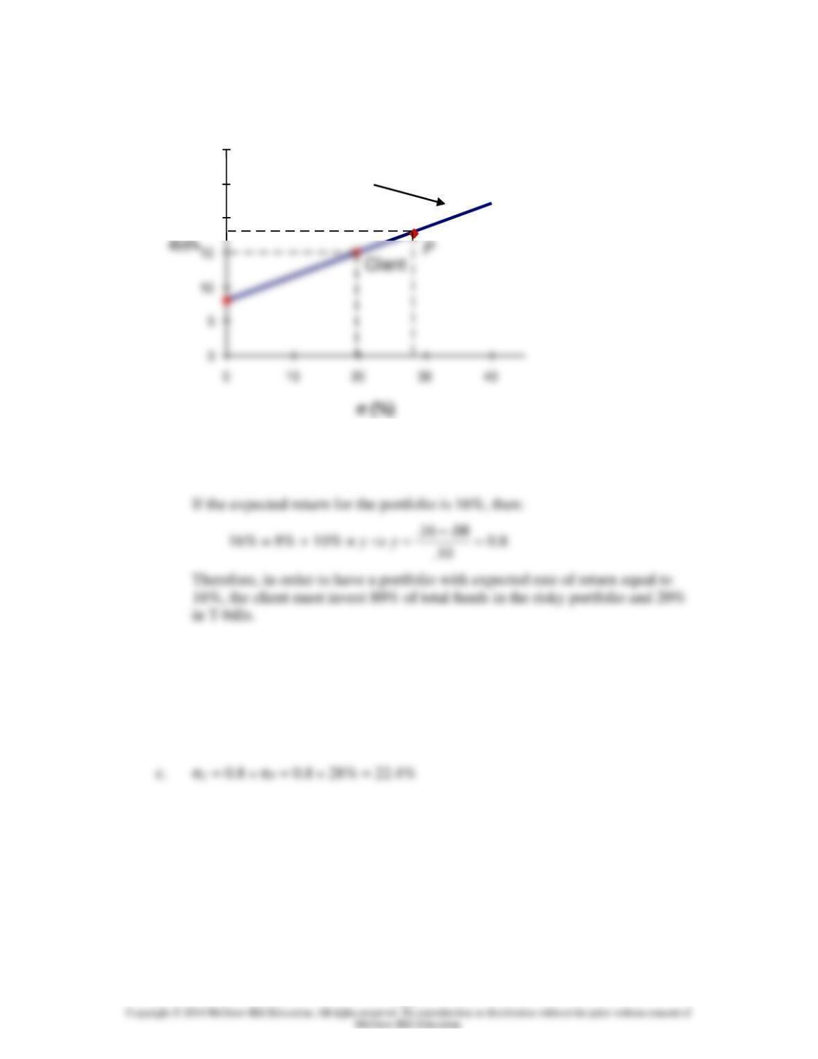
CAL (Slope = 0.3571)

17. a. E(rC) = rf + y × [E(rP) – rf] = 8 + y × (18 − 8)

b.

Client’s investment proportions:

20.0% in T-bills

0.8 × 25% =

20.0% in Stock A

0.8 × 32% =

25.6% in Stock B

0.8 × 43% =

34.4% in Stock C

6-

6

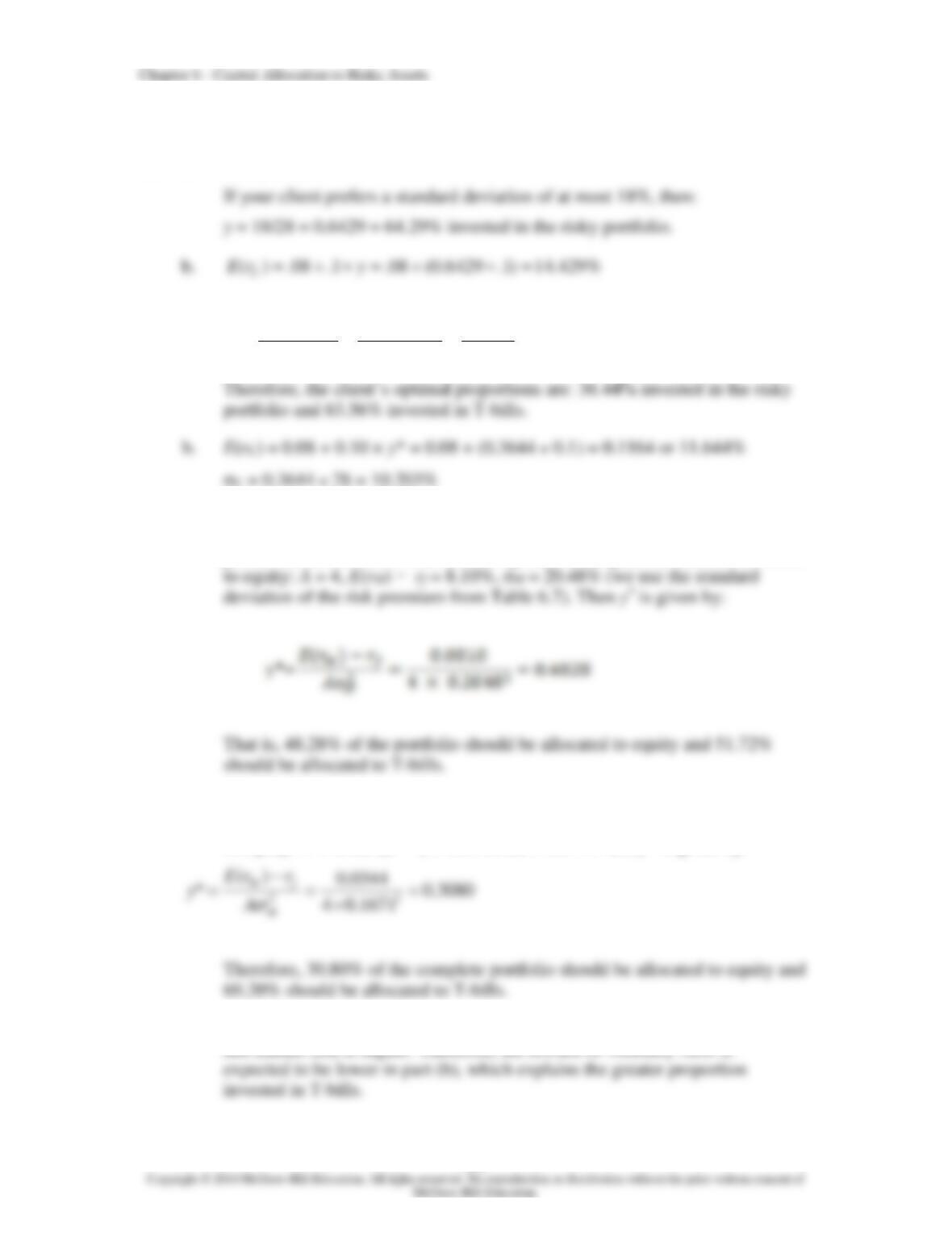
18. a. σC = y × 28%

19. a. y*

0.3644

0.2744

0.10

0.283.5

0.080.18

σ22 ==



−

=

−

=

P

fP

A

r)E(r

20. a. If the period 1926–2012 is assumed to be representative of future expected

performance, then we use the following data to compute the fraction allocated

b. If the period 1968–1988 is assumed to be representative of future expected

performance, then we use the following data to compute the fraction allocated

to equity: A = 4, E(rM) − rf = 3.44%, σM = 16.71% and y* is given by:

c. In part (b), the market risk premium is expected to be lower than in part (a)

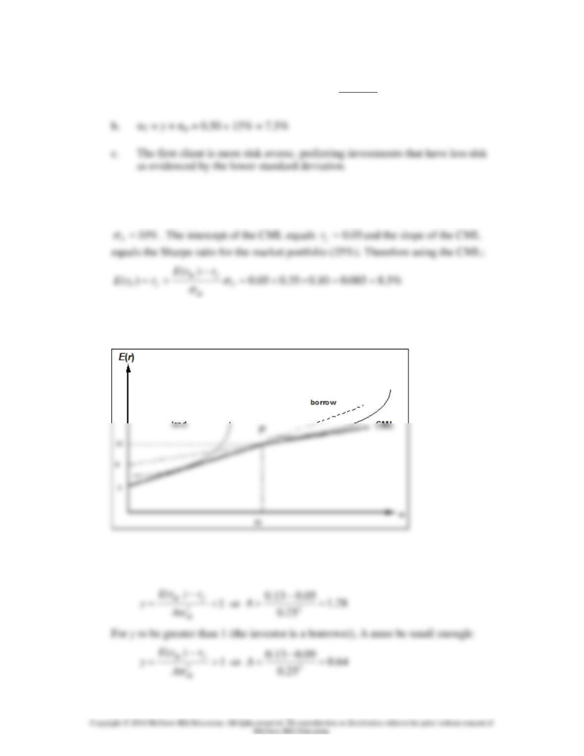
and market risk is higher. Therefore, the reward-to-volatility ratio is

Chapter 6 – Capital Allocation to Risky Assets

6-

7

21. a. E(rC) = 8% = 5% + y × (11% – 5%) 

.08 .05 0.5

.11 .05

y−

==

−

22. Johnson requests the portfolio standard deviation to equal one half the market

portfolio standard deviation. The market portfolio

20%

M



=

, which implies

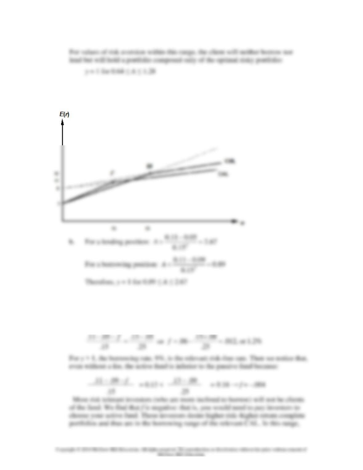
23. Data: rf = 5%, E(rM) = 13%, σM = 25%, and

B

f

r

= 9%

The CML and indifference curves are as follows:

24. For y to be less than 1.0 (that the investor is a lender), risk aversion (A) must be

large enough such that:

Chapter 6 – Capital Allocation to Risky Assets

6-

8

25. a. The graph for Problem 23 has to be redrawn here, with:

E(rP) = 11% and σP = 15%

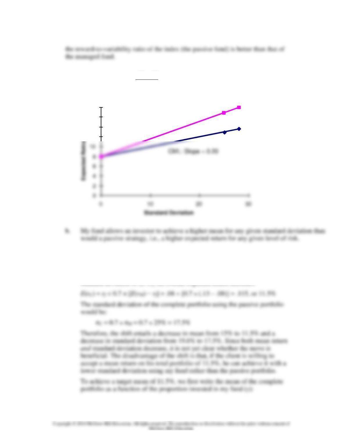
26. The maximum feasible fee, denoted f, depends on the reward-to-variability ratio.

For y < 1, the lending rate, 5%, is viewed as the relevant risk-free rate, and we solve

for f as follows:

Chapter 6 – Capital Allocation to Risky Assets

6-

9

27. a. Slope of the CML

.13 .08 0.20

.25

−

==

The diagram follows.

CML and CAL

10

12

14

16

18

CAL: Slope = 0.3571

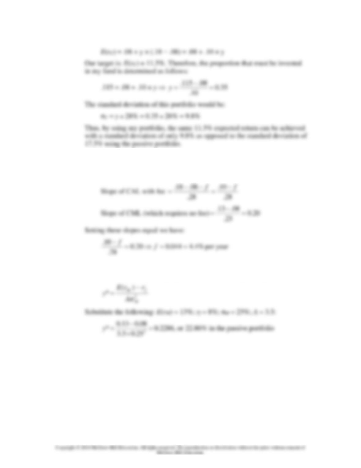
28. a. With 70% of his money invested in my fund’s portfolio, the client’s expected

return is 15% per year with a standard deviation of 19.6% per year. If he shifts

that money to the passive portfolio (which has an expected return of 13% and

standard deviation of 25%), his overall expected return becomes:

Chapter 6 – Capital Allocation to Risky Assets

6-

10

b. The fee would reduce the reward-to-volatility ratio, i.e., the slope of the CAL.

The client will be indifferent between my fund and the passive portfolio if the

slope of the after-fee CAL and the CML are equal. Let f denote the fee:

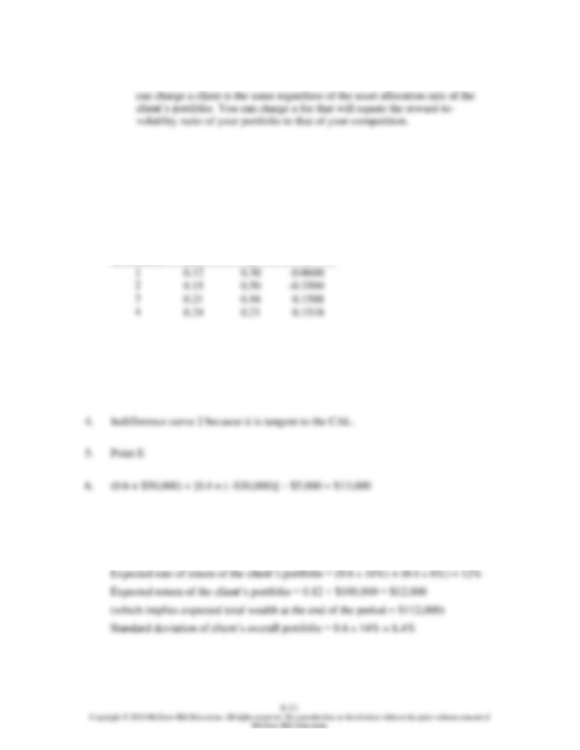
29. a. The formula for the optimal proportion to invest in the passive portfolio is:

Chapter 6 – Capital Allocation to Risky Assets

b. The answer here is the same as the answer to Problem 28(b). The fee that you

CFA PROBLEMS

1. Utility for each investment = E(r) – 0.5 × 4 × σ2

We choose the investment with the highest utility value, Investment 3.

Investment

Expected

return

E(r)

Standard

deviation



Utility

U

2. When investors are risk neutral, then A = 0; the investment with the highest utility

is Investment 4 because it has the highest expected return.

3. (b)

7. (b) Higher borrowing rates will reduce the total return to the portfolio and this

results in a part of the line that has a lower slope.

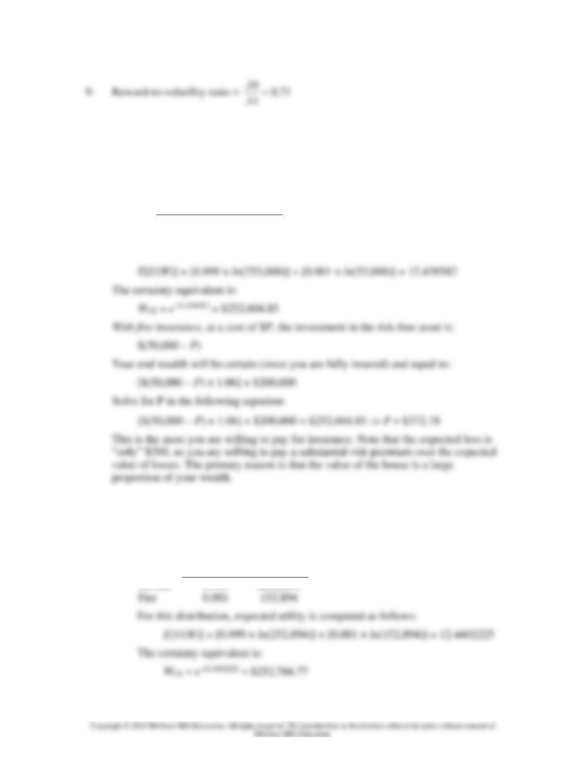
8. Expected return for equity fund = T-bill rate + Risk premium = 6% + 10% = 16%

Chapter 6 – Capital Allocation to Risky Assets

6-

12

CHAPTER 6: APPENDIX

1. By year-end, the $50,000 investment will grow to: $50,000 × 1.06 = $53,000

Without insurance, the probability distribution of end-of-year wealth is:

Probability

Wealth

No fire

0.999

$253,000

Fire

0.001

53,000

For this distribution, expected utility is computed as follows:

2. a. With insurance coverage for one-half the value of the house, the premium

is $100, and the investment in the safe asset is $49,900. By year-end, the

investment of $49,900 will grow to: $49,900 × 1.06 = $52,894

If there is a fire, your insurance proceeds will be $100,000, and the

probability distribution of end-of-year wealth is:

Probability

Wealth

No fire

0.999

$252,894

Chapter 6 – Capital Allocation to Risky Assets

6-

13

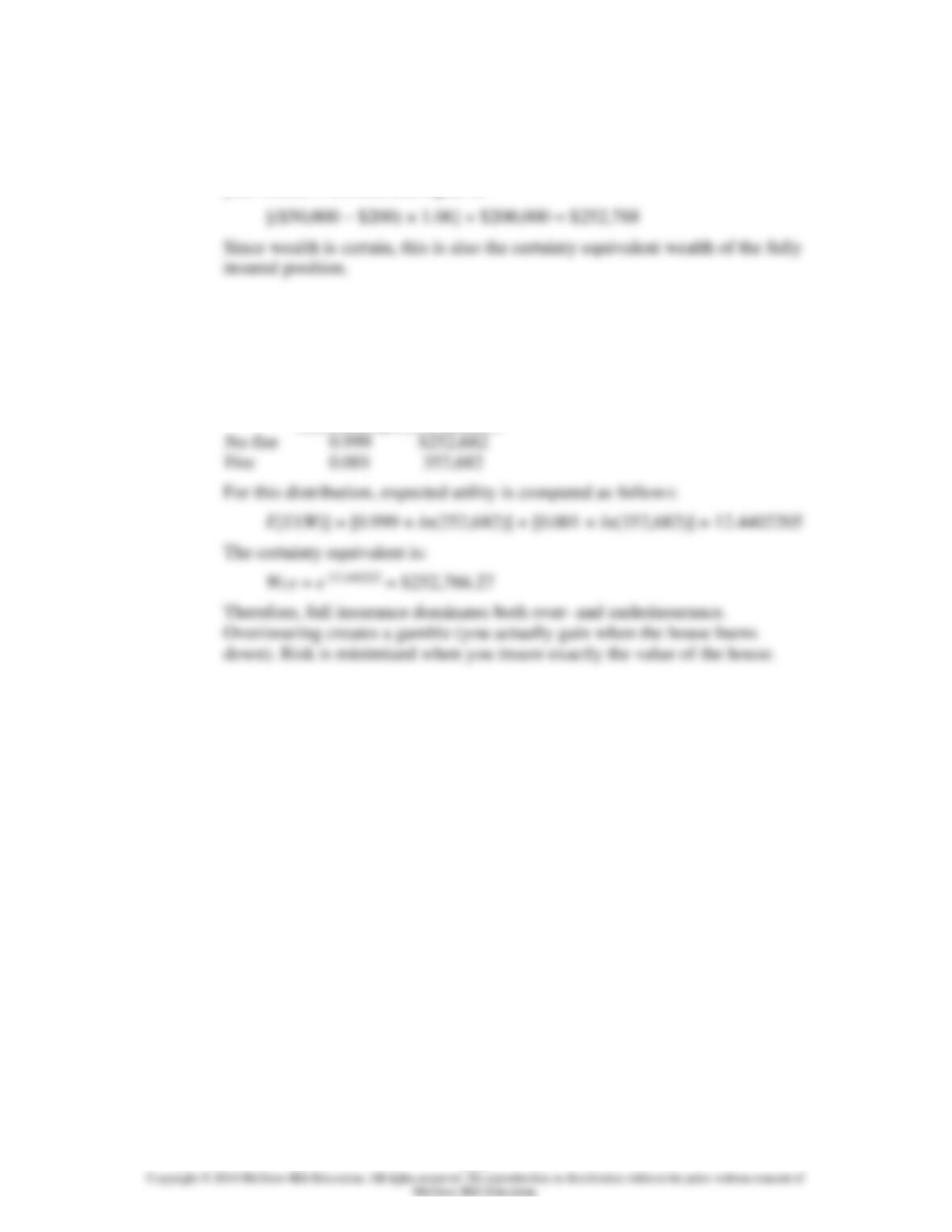
b. With insurance coverage for the full value of the house, costing $200, end-of-

year wealth is certain, and equal to:

c. With insurance coverage for 1½ times the value of the house, the premium

is $300, and the insurance pays off $300,000 in the event of a fire. The

investment in the safe asset is $49,700. By year-end, the investment of

$49,700 will grow to: $49,700 × 1.06 = $52,682

The probability distribution of end-of-year wealth is:

Probability

Wealth

No fire

$252,682