Chapter 5
Lesson 5-1 Classified Ads
Check Your Understanding (Example 1)
Check Your Understanding (Example 2)
Check Your Understanding (Example 3)
The cost is $38 for 1, 2, 3, or 4 lines. The cost is
38 6 25 4 when 4
⎩
Check Your Understanding (Example 4)
Check Your Understanding (Example 5)
Applications
1. Although consumers consider gas mileage,
2. 6 – 2 = 4, so there are 4 extra lines.
3. 4 – 3 = 1, so there is 1 extra line.
4. 7 – 4 = 3, so there are 3 extra lines.
5. x – m = x – m, so there are x – m extra lines.
6. $4,200 × 0.04 = $168
7. $18,500 × 0.05 = $925
$18,500 – $925 = $17,575
8. 27 – 20 = 7, so there are 7 extra words.
$18 + $0.35(7) = $18 + $2.45 = $20.45
9a. The cost is $46 for 200 characters or less. The
number of characters over 200, use the
expression x – 200.
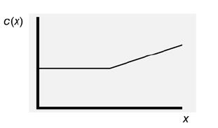
9b. The graph of the function is shown below.
9c. The cusp of the graph is when x = 200. The
value of c(x) when x = 200 is 46. The cusp is at
10. $6.50 × 4 = $26
11. $67 × 2.5 = $167.50
$48 + $5(2) = $48 + $10 = $58
12b. $52,900 × 0.08 = $4,232
14b. 1-line ad: $38
$38 – $38 = $0
= $38 + $18.75 = $56.75
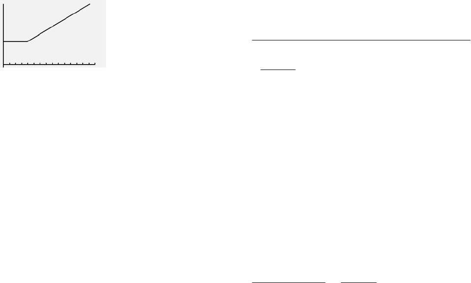
14d. The graph of the function is shown below.
14e. The cusp of the graph is when x = 4. The value
of c(x) when x = 4 is $38. The cusp is at
(4, $38).
15. Let x = number of lines in the ad. The cost is $29
.
29 when 5
29 6 75 5 when 5
() .( )
x
cx xx
≤
⎧
=⎨+− >
⎩
16a. The cost is $21.50 for three lines or less, and $5
16b. The cusp of the graph is when x = 3. The
17a. $11 × 2 = $22
17b. $11 × 3 + $5 × (5 – 3) =
$43
17c. The cost is $11 × x for 3 lines or less. The cost
lines over 3, use the expression x – 3.
.
33 5 3 when 3
() ()
cx xx
=⎨+− >
⎩
line over 5. To represent the number of lines
Lesson 5-2 Buy or Sell A Car
Check Your Understanding (Example 1)
= 35 100
6
Check Your Understanding (Example 2)
Mean: $1,200 + $1,650 + $1,500 + $2,000 +
Check Your Understanding (Example 3)
There are 6 values, so the median is the mean of
least value is $9,600. The fourth-least value is
2
2
Check Your Understanding (Example 4)
Check Your Understanding (Example 5)
By definition, 75% of the values are below Q3, so
Check Your Understanding (Example 6)
Check Your Understanding (Example 7)
From Example 7, an upper outlier is any value
Check Your Understanding (Example 8)

Applications
1. With the tremendous crunching and availability
2a. mean: 7 + 12 + 1 + 7 + 6 + 5 + 11 = 49; 49 ÷ 7
range: 12 – 1 = 11
2b. mean: 85 + 105 + 95 + 90 + 115 = 490; 490 ÷ 5
2c. mean: 10 + 14 + 16 + 16 + 8 + 9 + 11 + 12 + 3
= 99; 99 ÷ 9 = 11
mode: the data value 16 occurs 2 times; all other
range: 16 – 3 = 13
2d. mean: 10 + 8 + 7 + 5 + 9 + 10 + 7 = 56; 56 ÷ 7
= 8
modes are 7 and 10
range: 10 – 5 = 5
2e. mean: 45 + 50 + 40 + 35 + 75 = 245; 245 ÷ 5 =
third-least value, which is 45
mode
2f. mean: 15 + 11 + 11 + 16 + 16 + 9 = 78; 78 ÷ 6 =
13
+11 15
3. In 2a, the mean and median are the same, so
the data is not skewed. In 2b, the mean is 48
the same, so the data is not skewed.
4. $24,600 + $19,000 + $33,000 + $15,000 +
5a. $110 + $145 + $130 + $160 + $400 = $945
5b. There are 5 values, so the median is the third-
least value, which is $145
5c. Stephanie’s salary is much larger than the rest,
5d. The median is a better representation of the
data because of the outlier; 4 of the 5 data
values are below the mean.
6a. $59.00 + $71.00 + $50.00 = $180.00
6b. $59.00 + $71.00 + $50.00 = $180.00

7. 90 × 5 = 450
8. There are 52 weeks in a year, so he will work 50
9. 16 × 5 = 80
10. IQR = Q3 – Q1 = 110 – 50 = 60
11a. $210 + $210 + $320 + $200 + $300 + $10 +
11b. There are 14 values, so the median is the mean
11c. The data values $200, $210, and $300 each
occur 2 times; all other data values occur 1 time;
the modes are $200, $210, and $300
11d. Q2: median, which is $247.50
Q1: there are 7 values in the lower half of the
11e. IQR = Q3 – Q1 = $320 – $210 = $110
11f. $210 – 1.5($110) = $210 – $165 = $45
11g. $320 + 1.5($110) = $320 + $165 = $485
12a. Q2: there are 8 values, so Q2 is the mean of the
least value is $300. The fifth-least value is $350.
Q1: there are 4 values in the lower half of the
$180. The third-least value is $300.
data, so Q3 is the mean of the sixth-least (third-
greatest) and seventh-least (second-greatest)
12b. IQR = Q3 – Q1 = $425 – $240 = $185
12c. $240 – 1.5($185) = $240 – $277.50 = –$37.50
There are no values less than the lower-quartile
boundary.
12d. $425 + 1.5($185) = $425 + $277.50 = $702.50
⎝⎠
8
x
list price: 8
x
– 0.2 ⎛⎞
⎜⎟
x
, or .⎛⎞
⎜⎟
08 8
x
14. Answers vary. Numbers in the list must have a
16. Answers vary. Numbers in the list must have a
17. Answers vary. Sample: 3, 5, 10, 10, 10, 10, 12,
18. Answers vary. Sample: 1, 18, 20, 21, 22, 109.

19. The range is the greatest value minus the least
Lesson 5-3 Graph Frequency
Distributions
Check Your Understanding (Example 1)
Check Your Understanding (Example 2)
Check Your Understanding (Example 3)
Check Your Understanding (Example 4)
Check Your Understanding (Example 5)
Applications
1. You need facts–data–to back up any theory you
2. 1 + 4 + 3 + 1 + 7 = 16, so the 17th value is 750.
4. $1,200 – $540 = $660; the range is $660.
5. The sum of the frequencies, 33, is the total
6a.
$9,900 1
$10,800 2
$11,000 1
$12,500 2
$13,000 2
$23,000 1
6b. [(3 × $8,500) + (1 × $9,900) + (2 × $10,800) +
$11,000 + $25,000 + $26,000 + $14,500 +
$23,000) ÷ 13 = $156,600 ÷ 13 ≈ $12,038.46.
$8,500.
6e. $23,000 – $8,500 = $14,500
fourth-least values. The third-least value is
2 = $,18 400
2 = $9,200
Q3: there are 6 values in the upper half of the
values. The tenth-least value is $13,000. The
$, $,+13 000 13 000
6g. IQR = Q3 – Q1 = $13,000 – $9,200 = $3,800
6h. $13,000 + 1.5($3,800) = $13,000 + $5,700 =
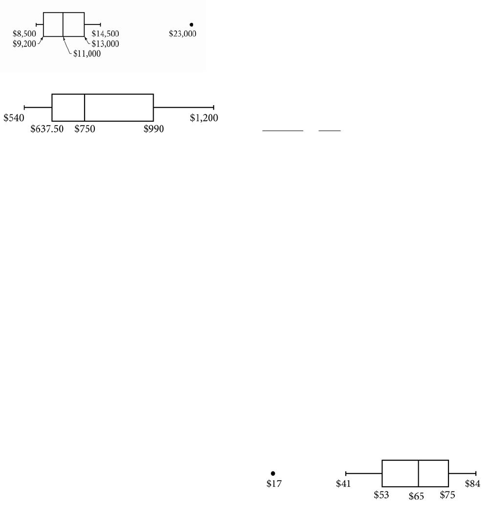
6k. The graph is shown below.
7a. The graph is shown below.
7b. If the data has an outlier, then a modified
7c. There are no single points outside the whiskers,
so there are no outliers.
8b. The 3 values below the mean are $18,000,
8c. There are 5 data values, so the median is the
8d. The 2 values below the median are $16,700 and
$15,900.
to calculate the linear regression equation.
The equation of the regression line is
9b. Use a graphing calculator to find the correlation
9c. Because the correlation coefficient, r, is close to
9d. y = –0.16(60,000) + 24,722.26
10a. There are 26 leaves in the table, so 26 students
were polled.
10b. (17 + 41 + 41 + 42 + 49 + 53 + 53 + 53 + 53 +
+ 75 + 75 + 77 + 82 + 82 + 83 + 84) ÷ 26 =
10c. There are 26 values, so the median is the mean
10d. The data value 53 occurs 5 times; all other data
10e. $84 – $17 = $67
10f. Q2: from part c, the median is $65.
$53.
data, so Q3 is the twentieth-least (seventh-
Q4: maximum value, which is $84
10g. $53 is Q1. By definition, 75% of the values are
10h. IQR = Q3 – Q1 = $75 – $53 = $22
10i. $53 is Q1. By definition, 25% of the values are
values are above Q3. 100% – 25% – 25% = 50%
10l. There is 1 data value ($17) below $20.
11c. The data value $226 occurs 3 times, all other
data values occur 2 times or 1 time, so the mode
is $226.

11d. There are 18 data values, so the median is the
mean of the ninth-least and tenth-least values.
2 = $379
2 = $189.50
12. The sum of the data is xy + 5w + 16 × 4 + 18v =
Lesson 5-4 Automobile Insurance
Check Your Understanding (Example 1)
Check Your Understanding (Example 2)
Check Your Understanding (Example 3)
Check Your Understanding (Example 4)
The insurance company pays a maximum of
Check Your Understanding (Example 5)
PIP insurance covers a maximum of $10,000 per
person.
28 × $10,000 = $280,000
Applications
1. Driving a car is a tremendous responsibility, and
2a. $32,000 > $25,000, so the insurance company
will pay the maximum coverage amount,
3c. $410 ÷ 2 = $205
4. $924
× 0.4 = $369.60
$924 × 0.3 = $277.20
7. The maximum for any one person is $50,000.
$23,000 + $500 + $50,000 = $73,500
9b. The fire hydrant is covered in full; $1,400.
10a. The sign is covered by property damage
insurance (PD).
10b. The sign is covered in full; y dollars (as long as
12
p
.
11b. 0.15 ⎛⎞
⎜⎟
⎝⎠
12
p
12a. The pole and minivan are covered by property
13. With the discount, the annual premium is
x – 0.35x.
The monthly premium is −035
12
.
x
x or 065
12
.
x
.
14a. With the discount, the annual premium is
quarterly payment = 09 +
4
xy
.
15b. With the increase, the annual premium is
x
17. Q2: there are 20 values, so the median is the
mean of the tenth-least and eleventh-least
(sixth-greatest) and sixteenth-least (fifth-
greatest) values, 60 and 61, so Q3 is 60.5.
Lesson 5-5 Linear Automobile
Depreciation
Check Your Understanding (Example 1)
Check Your Understanding (Example 2)
The intercepts are (0, D) and (T, 0).
Check Your Understanding (Example 3)
Check Your Understanding (Example 4)
The intercepts are (0, 18,495) and (9, 0).
Check Your Understanding (Example 5)
In the equation, let y = D and solve for x. The
expression will be the expression on the side of the
Check Your Understanding (Example 6)
You can include your monthly maintenance and
insurance costs with the monthly payment amount.
This will yield a slope that is greater than the one
depicted in the graph. Since the expense graph
Applications
1. This somewhat cynical quote compares the
monetary value of computers to that of
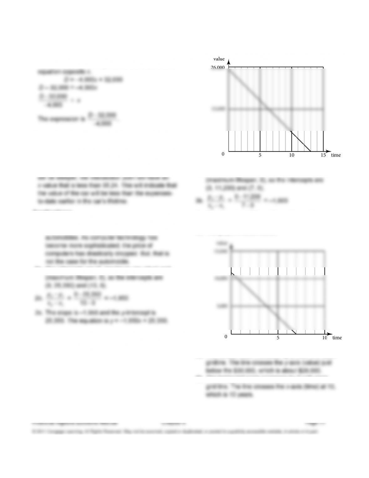
2a. The intercepts are (0, maximum car value) and
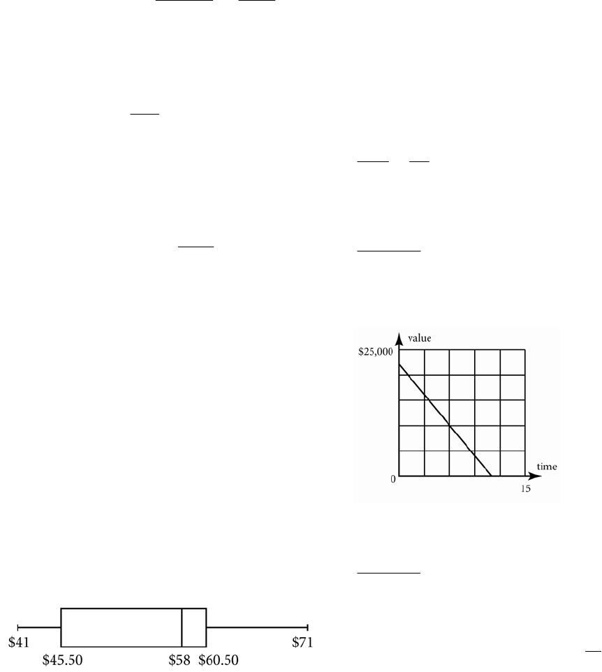
2d. The graph is shown below.
3a. The intercepts are (0, maximum car value) and
3c. The slope is –1,600 and the y-intercept is
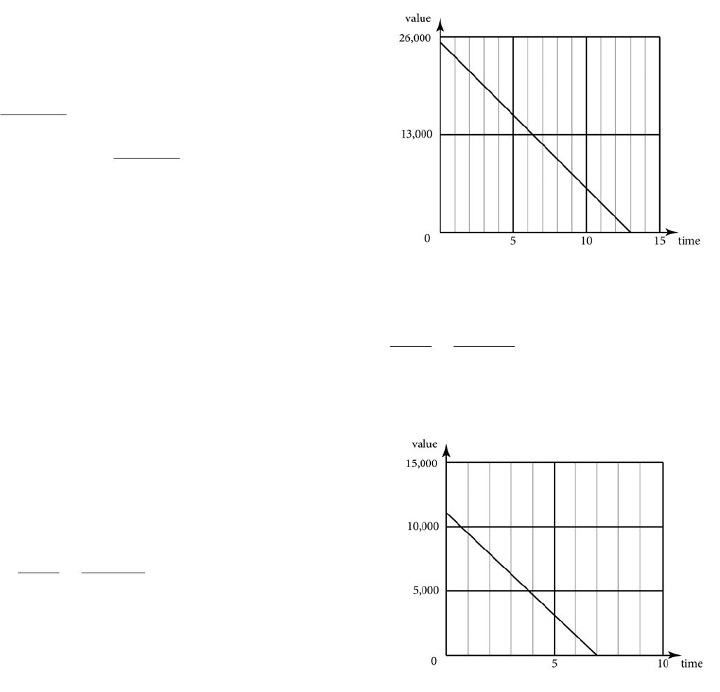
11,200. The equation is y = –1,600x + 11,200.
3d. The graph is shown below.
4a. The vertical scale increases by $7,000 with each
4b. The horizontal scale increases by 2 with each
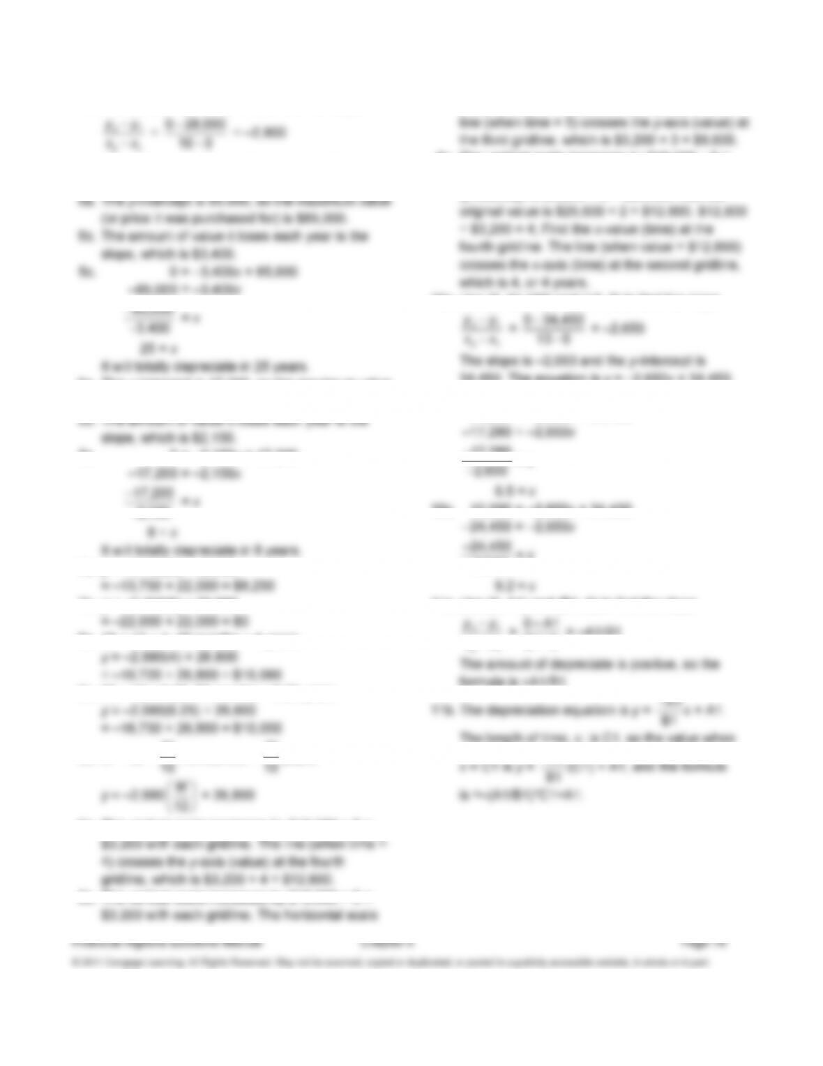

4c. Use (0, 28,000) and (10, 0) to find the slope.
x
The slope is –2,800 and the y-intercept is
28,000. The equation is y = –2,800x + 28,000.
6a. The y-intercept is 17,200, so the maximum value
(or its original price) is $17,200.
5c. 0 = –2,150x + 17,200
2 150
−
, = x
7a. y = –2,750(5) + 22,000
7b. y = –2,750(8) + 22,000
8a. 48 ÷ 12 = 4; 48 months = 4 years
8b. 75 ÷ 12 = 6.25; 75 months = 6.25 years
8c. M ÷ 12 = 12
M; M months = 12
Myears
9a. The vertical scale increases by $16,000 ÷ 5 =
9b. The vertical scale increases by $16,000 ÷ 5 =
increases by 4 ÷ 2 = 2 with each gridline. The
9c. The vertical scale increases by $16,000 ÷ 5 =
$3,200 with each gridline. The maximum value
(y-intercept is $3,200 × 8 = $25,600. Half the
10a. Use (0, 34,450) and (13, 0) to find the slope.
−
−
y
x
34,450. The equation is y = –2,650x + 34,450.
10b. 34,560 ÷ 2 = 17,280
17,280 = –2,650x + 34,450
17 280
−
,
10c. 10,000 = –2,650x + 34,450
2 650
−
,= x
11a. Use (0, A1) and (B1, 0) to find the slope.
−
−
y
x
x = 0A1
B1 0
−
= –A1/B1
formula is =A1/B1.
A
The length of time, x, is C1, so the value when
A
1
−
12a. The depreciation equation is y = –B1x + A1.
0 = –B1x + A1
12b. The depreciation equation is y = –B1x + A1.
D1 = –B1x + A1
12c. Find the complement of the percent: 100 – E1.
((100 – E1)/100)*A1 = –B1x + A1
13a. Amount financed = $54,000 – $8,000 = $46,000.
Use the monthly payment formula:
12
t
rr
⎛⎞⎛ ⎞
12(4)
0.04875 0.04875
$46,000 1
12 12
0.04875
11
12
⎛⎞⎛ ⎞
+
⎜⎟⎜ ⎟
⎝⎠⎝ ⎠
=
⎛⎞
+−
⎜⎟
⎝⎠
M
M ≈ $1,056.74
The monthly payment is $1,056.74.
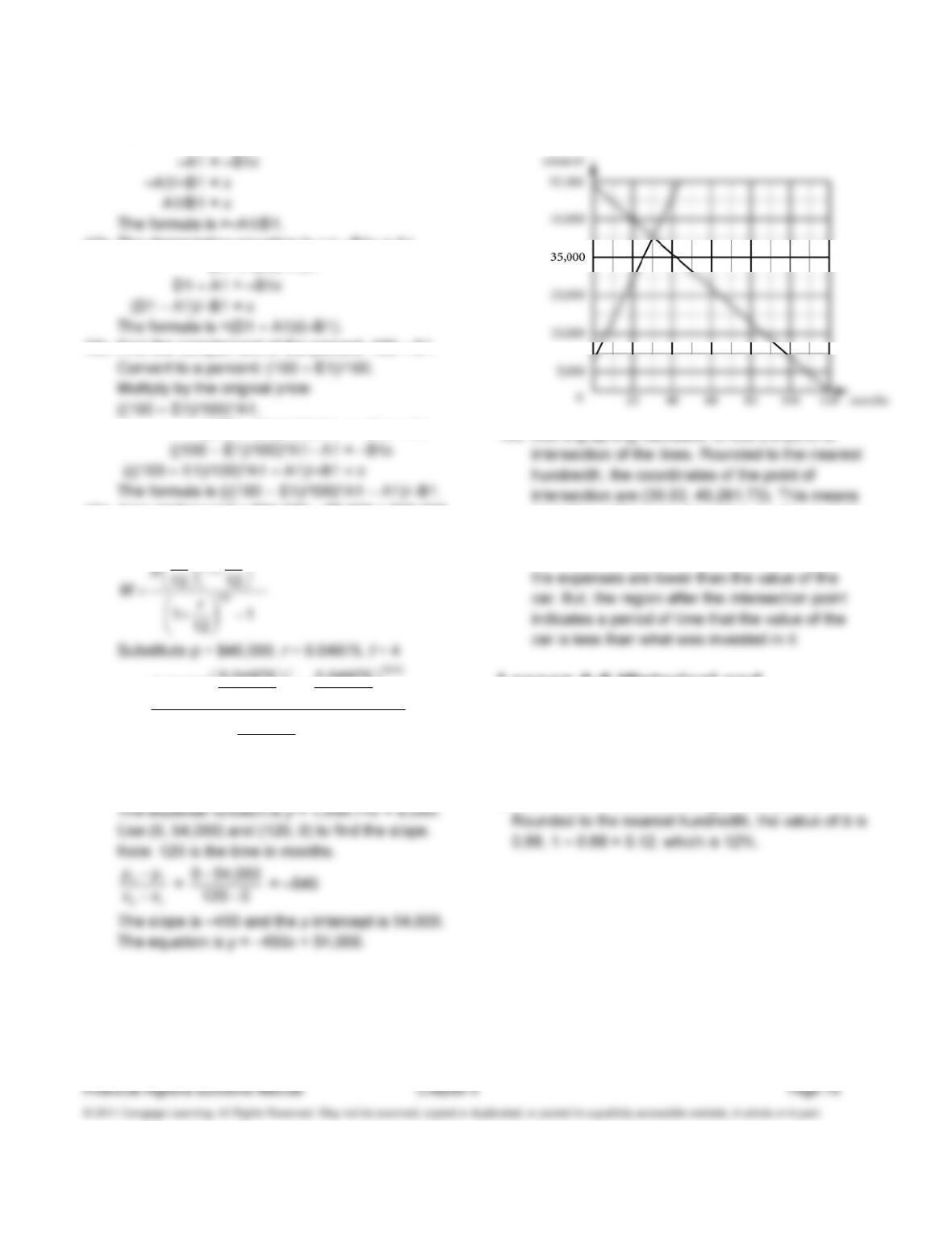
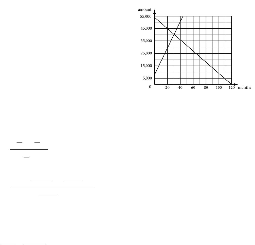
13b. The graph is shown below.
13c. Use a graphing calculator to find the point of
that after a little more than 30.5 months, both the
expenses-to-date and the car’s value are the
same. In the region before the intersection point,
Lesson 5-6 Historical and
Exponential Depreciation
Check Your Understanding (Example 1)
The graph would be closer to the data points.
Check Your Understanding (Example 2)