Unlock document.
This document is partially blurred.
Unlock all pages and 1 million more documents.
Get Access
Chapter 05 - Risk and Return: Past and Prologue
CHAPTER 05
RISK AND RETURN: PAST AND PROLOGUE
1. The 1% VaR will be less than –30%. As percentile or probability of a return declines so
3. The excess return on the portfolio will be the same as long as you are consistent: you
can use either real rates for the returns on both the portfolio and the risk-free asset, or
4. Decrease. Typically, standard deviation exceeds return. Thus, an underestimation of 4%
5. Using Equation 5.10, we can calculate the mean of the HPR as:
Using Equation 5.11, we can calculate the variance as:
Var(r) = 2 = ∑p(s) [ r(s)
𝑆
𝑠=1 – E(r)]2
6. We use the below equation to calculate the holding period return of each scenario:
HPR = Ending Price - Beginning Price + Cash Dividend
Beginning Price
a. The holding period returns for the three scenarios are:
Chapter 05 - Risk and Return: Past and Prologue
Recession: (34 – 40 + 0.50)/40 = –0.1375 = –13.75%
E(HPR) = ∑p(s) r(s)
𝑆
𝑠=1
Var(HPR) = ∑p(s) [ r(s)
𝑆
𝑠=1 – E(r)]2
b. E(r) = (0.5 8.75%) + (0.5 4%) = 6.375%
7. a. Time-weighted average returns are based on year-by-year rates of return.
Year
Return = [(Capital gains + Dividend)/Price]
2010-2011
(110 – 100 + 4)/100 = 0.14 or 14.00%
b.
Date
1/1/2010
1/1/2011
1/1/2012
1/1/2013
Chapter 05 - Risk and Return: Past and Prologue
8. a. Given that A = 4 and the projected standard deviation of the market return =
20%, we can use the below equation to solve for the expected market risk
premium:
b. Solve E(rM) – rf = 0.09 = AM2 = A (0.20) , we can get
9. From Table 5.3, we find that for the period 1926 – 2013, the mean excess return for
10. To answer this question with the data provided in the textbook, we look up the
historical excess returns of the large stocks, small stocks, and Treasury Bonds for
1926-2013 from Table 5.3.
Excess Return – Arithmetic Average
11.
a. The expected cash flow is: (0.5 $50,000) + (0.5 $150,000) = $100,000
With a risk premium of 10%, the required rate of return is 15%. Therefore, if
the value of the portfolio is X, then, in order to earn a 15% expected return:
b. If the portfolio is purchased at $86,957, and the expected payoff is $100,000, then
the expected rate of return, E(r), is:
c. If the risk premium over T-bills is now 15%, then the required return is:
d. For a given expected cash flow, portfolios that command greater risk premiums
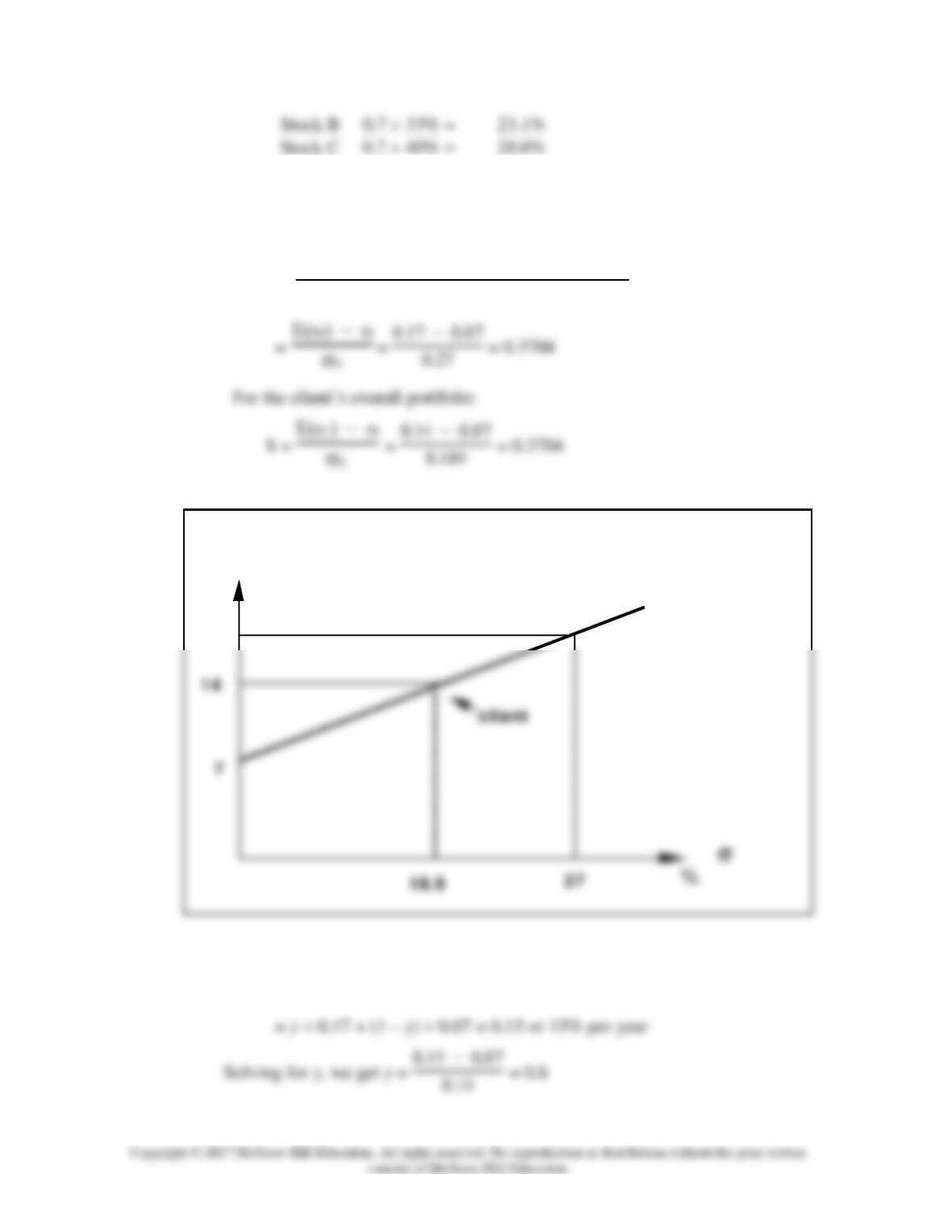
12. a. Allocating 70% of the capital in the risky portfolio P, and 30% in risk-free asset,
the client has an expected return on the complete portfolio calculated by adding
up the expected return of the risky proportion (y) and the expected return of the
proportion (1 - y) of the risk-free investment:
b. The investment proportions of the client’s overall portfolio can be calculated by
the proportion of risky portfolio in the complete portfolio times the proportion
allocated in each stock.
Chapter 05 - Risk and Return: Past and Prologue
c. We calculate the reward-to-variability ratio (Sharpe ratio) using Equation 5.14.
For the risky portfolio:
S = Portfolio Risk Premium
Standard Deviation of Portfolio Excess Return
13.
a. E(rC) = y E(rP) + (1 – y) rf
E(r)
17 P CAL ( slope=.3704)
%
Chapter 05 - Risk and Return: Past and Prologue
b. The investment proportions of the client’s overall portfolio can be calculated by
the proportion of risky asset in the whole portfolio times the proportion
allocated in each stock.
Security
Investment
Proportions
T-Bills
20.0%
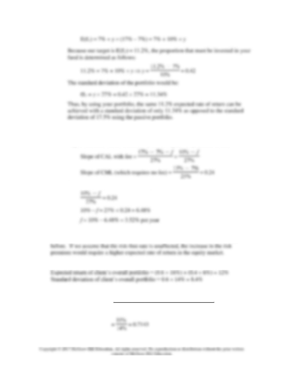
c. The standard deviation of the complete portfolio is the standard deviation of the
risky portfolio times the fraction of the portfolio invested in the risky asset:
14.
a. Standard deviation of the complete portfolio= C = y 0.27
If the client wants the standard deviation to be equal or less than 20%, then:
15.
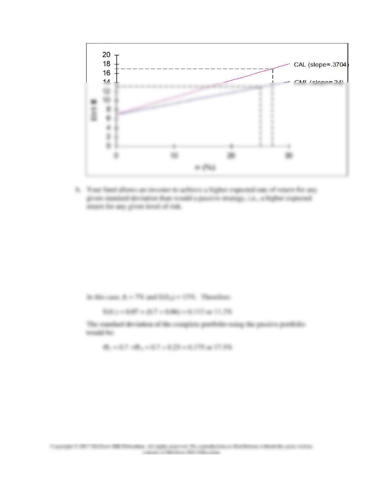
a. Slope of the CML = E(rM) - rf
M
= 0.13 - 0.07
0.25 = 0.24
See the diagram below:
Chapter 05 - Risk and Return: Past and Prologue
16.
a. With 70% of his money in your fund's portfolio, the client has an expected rate
of return of 14% per year and a standard deviation of 18.9% per year. If he
shifts that money to the passive portfolio (which has an expected rate of return
of 13% and standard deviation of 25%), his overall expected return and standard
deviation would become:
E(rC) = rf + 0.7 E(rM) – rf]
Therefore, the shift entails a decline in the mean from 14% to 11.2% and a decline
in the standard deviation from 18.9% to 17.5%. Since both mean return and
standard deviation fall, it is not yet clear whether the move is beneficial. The
disadvantage of the shift is apparent from the fact that, if your client is willing to
accept an expected return on his total portfolio of 11.2%, he can achieve that
return with a lower standard deviation using your fund portfolio rather than the
passive portfolio. To achieve a target mean of 11.2%, we first write the mean of
the complete portfolio as a function of the proportions invested in your fund
portfolio, y:
Chapter 05 - Risk and Return: Past and Prologue
b. The fee would reduce the reward-to-variability ratio, i.e., the slope of the CAL.
Clients will be indifferent between your fund and the passive portfolio if the
slope of the after-fee CAL and the CML are equal. Let f denote the fee:
Setting these slopes equal and solving for f:
17. Assuming no change in tastes, that is, an unchanged risk aversion, investors perceiving
higher risk will demand a higher risk premium to hold the same portfolio they held
18. Expected return for your fund = T-bill rate + risk premium = 6% + 10% = 16%
19. Reward to volatility ratio = Portfolio Risk Premium
Standard Deviation of Portfolio Excess Return
20.
Excess Return (%)
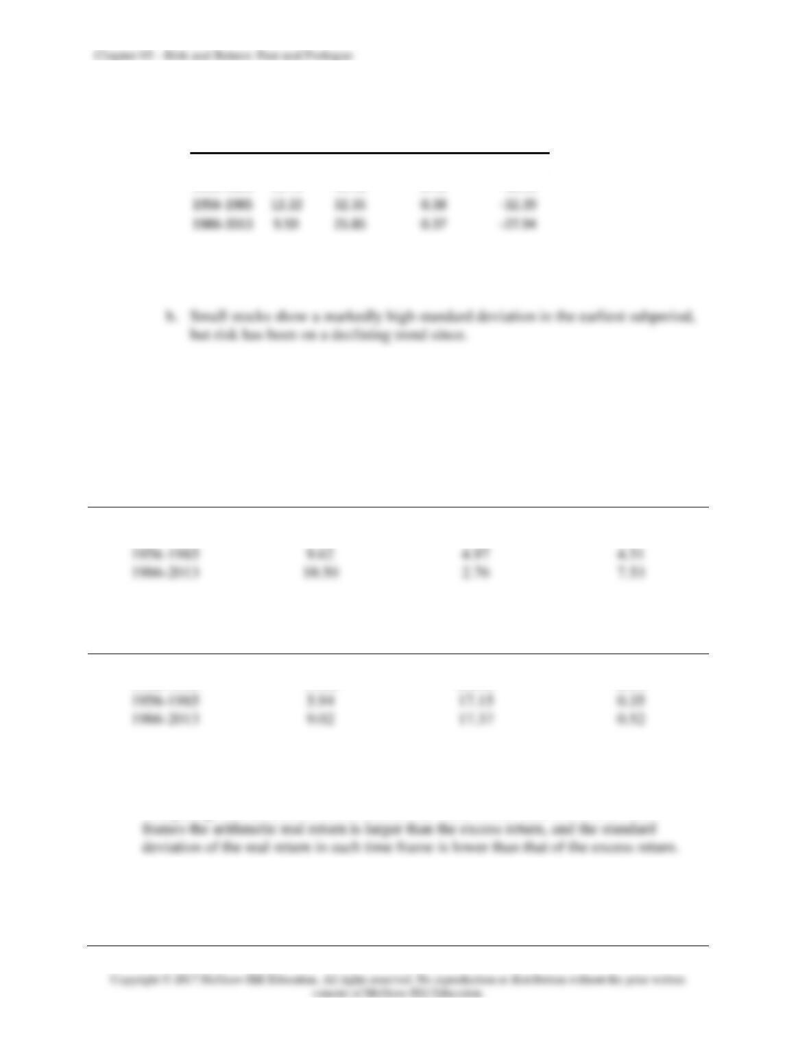
a. In three out of four time frames presented, small stocks provide worse ratios
than large stocks.
21. For geometric real returns, we take the geometric average return and the real geometric
return data from Table 5.3 and then calculate the inflation in each time frame using the
equation: Inflation rate = (1 + Nominal rate)/(1 + Real rate) – 1.
Geometric Real Returns (%) – Large Stocks
Average
Inflation
Real Return
1926-2013
9.88
2.97
6.71
1926-1955
9.66
1.36
8.18
Risk Return Ratio – Large Stocks
Arithmetic Real
Return
Std Dev
Real Return to Risk
1926-2013
8.71
20.19
0.43
1926-1955
11.20
25.18
0.44
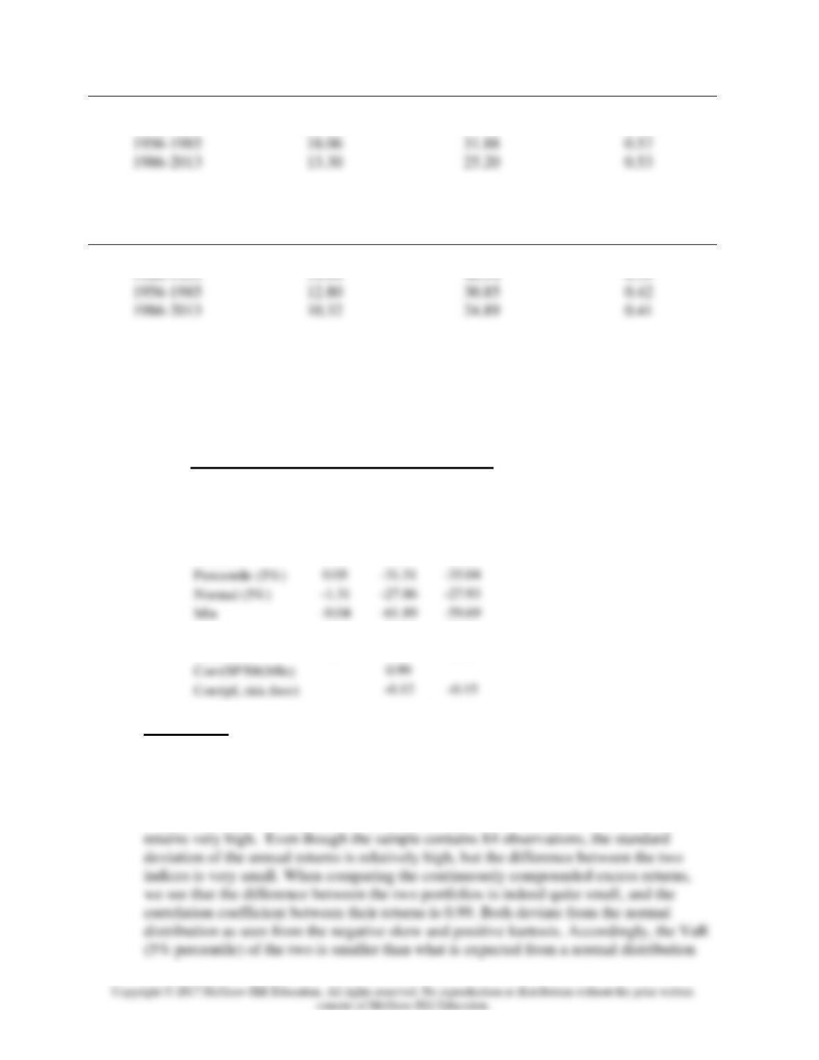
The VaR is not calculated.
Comparing with the excess return statistics in Table 5.4, in three out of four time
22.
Nominal Returns (%) – Small Stocks
Nominal Return
Std Dev
Return to Risk
Average Std Dev Sharpe Ratio 5% VaR
1926-2013 13.94 37.29 0.37 -36.96
1926-1955 19.73 49.46 0.40 -46.25
Chapter 05 - Risk and Return: Past and Prologue
1926-2013
17.48
36.73
0.48
1926-1955
20.82
49.10
0.42
Real Return (%) – Small Stocks
Arithmetic Real
Return
Std Dev
Return to Risk
1926-2013
14.14
36.08
0.39
The VaR is not calculated.
Comparing the nominal rate with the real rate of return, the real rates in all time frames
and their standard deviation are lower than those of the nominal returns.
23.
Results T Bill
S&P 500 Market
Average 3.56 5.57 5.63
SD 2.96 20.33 20.41
Skew 0.90 -0.87 -0.88
Kurtosis 0.70 1.06 0.92
Max 13.73 43.24 45.13
Serial corr 0.91 0.05 0.06
Comparison
The combined market index represents the Fama-French market factor (Mkt). It is
better diversified than the S&P 500 index since it contains approximately ten times as
many stocks. The total market capitalization of the additional stocks, however, is
relatively small compared to the S&P 500. As a result, the performance of the value-
weighted portfolios is expected to be quite similar, and the correlation of the excess
Chapter 05 - Risk and Return: Past and Prologue
with the same mean and standard deviation. This is also indicated by the lower
minimum excess return for the period. The serial correlation is also small and
indistinguishable across the portfolios.
CFA 1
CF 2
CFA 3
CFA 4
Answer: Investment 3.
For each portfolio: Utility = E(r) – (0.5 4 2)
Investment
E(r)
Utility
1
0.12
0.30
-0.0600
3
0.21
0.16
0.1588
We choose the portfolio with the highest utility value.
CFA 5
CFA 6
CFA 7
Answer:
Chapter 05 - Risk and Return: Past and Prologue
CFA 8
Answer:
CFA 9
Answer:
CFA 10
Answer:
The probability is 0.5 that the state of the economy is neutral. Given a neutral
CFA 11
Answer:


