Unlock document.
This document is partially blurred.
Unlock all pages and 1 million more documents.
Get Access
Chapter 05 - Risk and Return: Past and Prologue
CHAPTER FIVE
RISK AND RETURN: PAST AND PROLOGUE
CHAPTER OVERVIEW
This chapter introduces the concept of risk and return. To induce rational investors to accept
more risk they must be promised a sufficiently large enough return to overcome their risk
aversion. The concept of excess returns or risk premiums is developed and Value at Risk (VaR)
and the Sharpe performance measure are introduced. The primary focus of the chapter however
LEARNING OBJECTIVES
After covering this chapter, the student should be able to calculate ex post and ex ante risk and
return statistical measures, such as holding-period returns, average returns, expected returns, and
standard deviations. Readers should understand the differences between time-weighted and
dollar-weighted returns, geometric and arithmetic averages and have some idea when to use
each. Students will also gain a basic understanding of returns and risk of various asset classes
and understand that securities that offer higher returns have higher risk. In addition, the student
CHAPTER OUTLINE
1. Rates of Return
PPT 5-2 through PPT 5-7
The PPT begins by calculating holding period returns or HPRs and discusses why we calculate
returns and sometimes annualize them. Annualizing with and without compounding is
illustrated. This should be a review of the students’ basic finance course.
There are several methods for averaging returns over multiple periods. The first choice with
2. Inflation and Real Rates of Return
PPT 5-8 through PPT 5-11
The concept of real versus nominal rates and the Fisher Effect are presented. The reason for
needing the exact version of the Fisher Effect is given in a hidden slide with a hyperlink so that
the instructor may use it or not. Note that the approximation version and the exact version of the
Fisher Effect will diverge at higher rates of inflation. The effects of inflation and taxes on an
investor’s return are illustrated. Note that since taxes are paid out of nominal earnings you must
take taxes out of the nominal return before finding the real return.
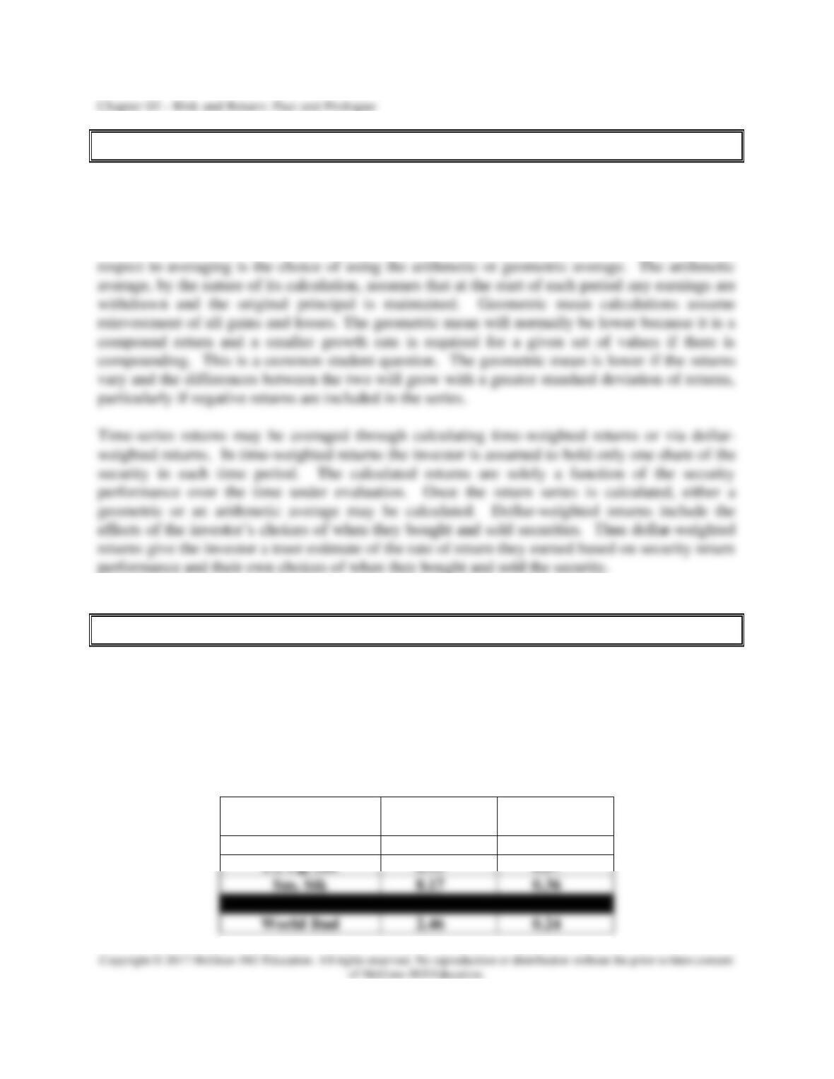
Historical Real Returns & Sharpe Ratios 1926-2008
Series
Real
Returns%
Sharpe Ratio
World Stk
6.00
0.37
US Lg. Stk
6.13
0.37
Chapter 05 - Risk and Return: Past and Prologue
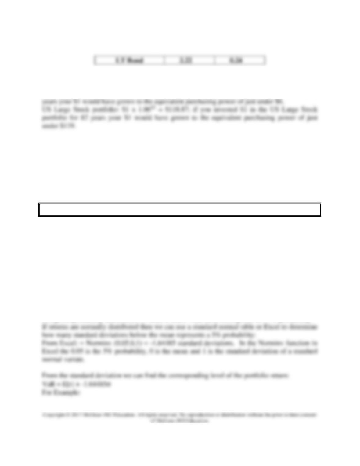
Stocks have much higher real returns over long time periods. To illustrate what this implies we
can calculate the following future values:
LT Bond portfolio: $1 x 1.02282 = $5.96; if you had invested $1 in the LT Bond portfolio for 82
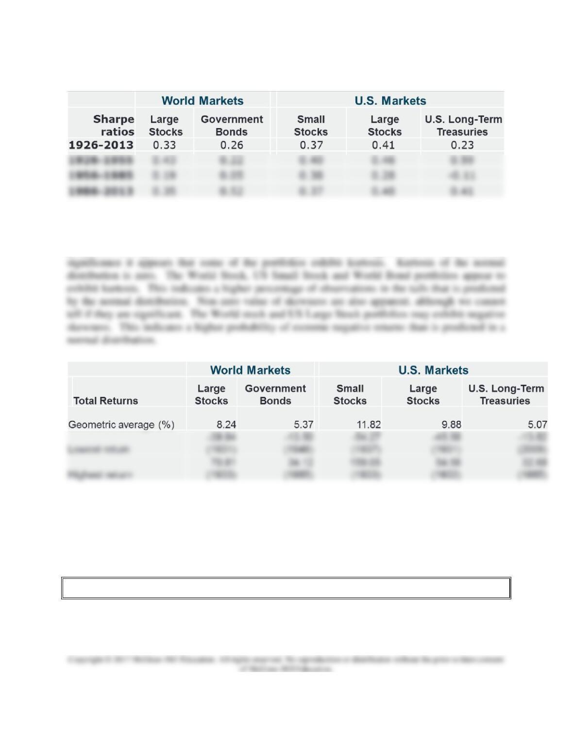
The Sharpe ratio is a measure of the excess return per unit of standard deviation risk. It literally
measures the return per unit of risk taken. Higher Sharpe ratios indicate better the performance
for that asset class. Notice that the Sharpe ratios are higher for the three-stock portfolios than the
bonds. Thus the stocks offered a higher rate of return per unit of risk. Does that mean investors
should not hold bonds? No, adding bonds to a stock portfolio will eliminate proportionally more
risk than the return sacrificed and can lead to higher Sharpe ratios.
3. Risk and Risk Premiums
PPT 5-12 through PPT 5-21
This section begins by illustrating calculations of expected returns and standard deviation ex-ante
for individual securities via scenario analysis. Ex-post average return and standard-deviation
calculations are also provided. Basic characteristics of probability distributions are then covered
including definitions of mean, variance, skew and kurtosis. For distributions that are skewed, the
median and mean returns are different. For normal distributions the mean and variance or
standard deviation are sufficient statistics to characterize the distribution.
Value at Risk
Value at Risk attempts to answer the following question:
How many dollars can I expect to lose on my portfolio in a given time period at a given level of
probability?
The typical probability used is 5%.
In a given probability distribution we need to know what HPR corresponds to a 5% probability.
Chapter 05 - Risk and Return: Past and Prologue
A $500,000 stock portfolio has an annual expected return of 12% and a standard deviation of
35%. What is the portfolio VaR at a 5% probability level?
VaR = 0.12 + (-1.64485 * 0.35)
VaR is an easily understood quality-control measure. Investment oversight boards can determine
whether this loss is acceptable given the portfolio’s goals. The VaR calculation does not require
VaR versus Standard Deviation:
For normally distributed returns VaR is equivalent to standard deviation (although VaR is
typically reported in dollars rather than in % returns). VaR adds value as a risk measure when
Risk Premium and Risk Aversion
The risk-free rate is the rate of return that can be earned with certainty. The risk premium is the
difference between the expected return of a risky asset and the risk-free rate. The risk premium
4. The Historical Record
PPT 5-22 through PPT 5-24
Chapter 05 - Risk and Return: Past and Prologue
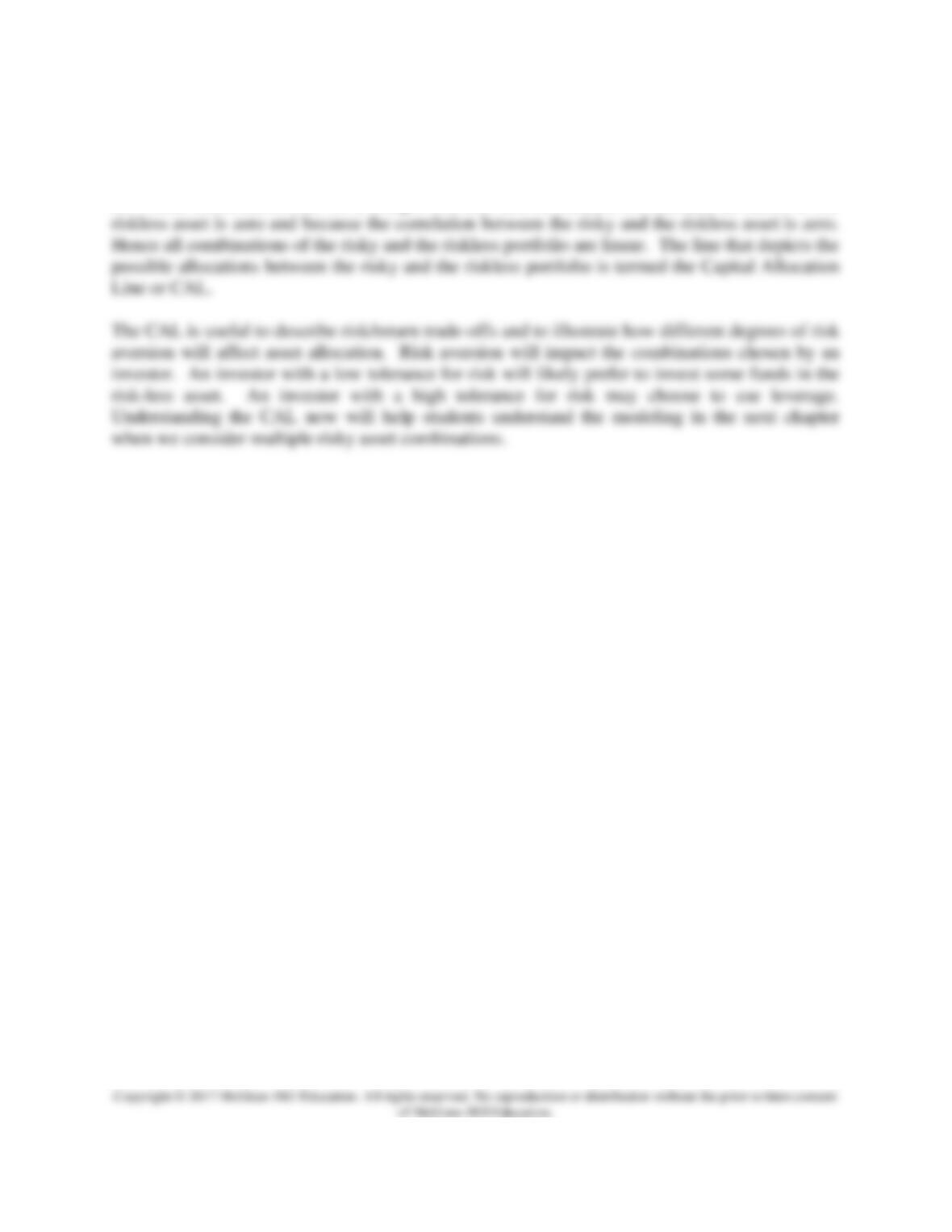
The geometric mean is the best measure of the compound historical rate of return. Nevertheless
the arithmetic average is the best measure of the expected return. Notice the greater divergence
of the GAR and AAR for small stocks. This is because of the high variance and the higher
proportion of negative returns in the small stock portfolio. Although we don’t have statistical
5. Asset Allocation across Risky and Risk-Free Portfolios
PPT 5-25 through PPT 5-29
Chapter 05 - Risk and Return: Past and Prologue
Investors can choose to hold risky and riskless assets. We may consider investments in a money
market mutual fund as a proxy for the riskless investments that an investor might actually engage
in. These combinations fall on a straight line (see below) because the standard deviation of the
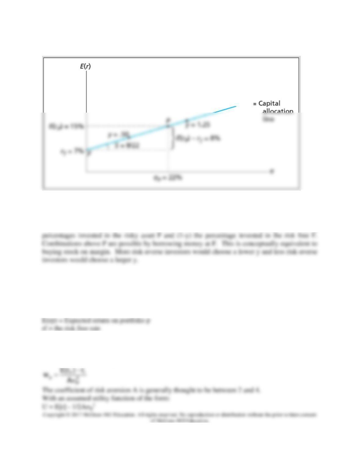
Chapter 05 - Risk and Return: Past and Prologue
The expected return is on the vertical axis and the standard deviation of the total portfolio is on
the horizontal axis. With all of your money in the risk free asset (F) you will have a 7% return
and a zero standard deviation. With 100% of your money in the risky asset you will have a 15%
expected return and a 22% standard deviation. Combinations (y) less than one represent varying
Quantifying Risk Aversion
Some efforts have been made to quantify risk aversion (A). The text assumes that the risk
premium or excess return is proportional to the product of the risk aversion level A and the
variance of the portfolio.
( )
2
p
fp A5.0rrE =−
0.5 = Scale factor
A x p2 = Proportional risk premium
A larger A indicates that the investor requires more return to bear risk. In the asset allocation
decision the optimal weight in the risky portfolio P (WP) is:
CAL
Chapter 05 - Risk and Return: Past and Prologue
The A term can used to create indifference curves. Indifference curves describe different
combinations of return and risk that provide equal utility (U) or satisfaction. Indifference curves
6. Passive Strategies and the Capital Market Line
PPT 5-30 through PPT 5-31
In a passive strategy the investor makes no attempt to either find undervalued strategies or
actively switch their asset allocations. Investing in a broad stock index and a risk-free
investment is an example of a passive strategy. The CAL that employs the market (or an index
Excess Returns and Sharpe Ratios Implied by the CML
The average risk premium implied by the CML for large common stocks over the entire time
period is 7.86%. But the subperiod variation and the large standard deviation indicate that


