
(c) Is the average monthly rate of return of 33.33% indicative of the performance of Smith
& Jones? If not, what would be a more appropriate measure?
The 33.33% monthly rate of return is not indicative of the performance of Smith & Jones. A
more appropriate measure would be the time-weighted rate of return or the dollar-weighted
rate of return.
whereRTis the time-weighted rate of return, RPkis the return for subperiod k for k = 1, . . . , N,and
Nis the number of subperiods.
In our problem, we have the portfolio returns for the client of RP1 = −50%, RP2 = 200%, RP3 =
−50% and RP4 = 33.33%, for months 1, 2, 3, and 4, respectively. Solving for N = 4,
the time-weighted rate of return is:
If the time-weighted rate of return is 0% per month, one dollar invested in the portfolio at the
beginning of month 1 would have grown at a rate of 0% per month during the four-month
evaluation period. This answer is consistent with the fact that Smith and Jones’ client began with
Cash flows, referred to above, are defined as follows:
(1) A cash withdrawal is treated as a cash inflow. So, in the absence of any cash contribution
(2) A cash contribution is treated as a cash outflow. Consequently, in the absence of any cash

(3) If there are both cash contributions and cash withdrawals for a given time period, then the cash
flow is as follows for that time period: If cash withdrawals exceed cash contributions, then
The dollar-weighted rate of return is simply an internal rate-of-return calculation and hence it is
also called the internal rate of return. The general formula for the dollar-weighted return is:
V0 =
( ) ( )
11
2
111
NN
N
DDD
CV
CC
RRR
+
+ + +
+++
Notice that it is not necessary to know the market value of the portfolio for each subperiod to
determine the dollar-weighted rate of return.
For our problem, we have: V0 = $100 million, N = 4, C1 = $0 million, C2 = $0 million,
C3 = $0 million, C4 = $0 million, and V4 = $100 million. Given these values, RDis the interest rate
that satisfies the below equation:
$100,000,000 =
( ) ( ) ( ) ( )
2 3 4
$0 $0 $0 $0 $100,000,000
11 1 1
DD D D
RR R R
+
+ + +
++ + +
➔
Another way of looking at this problem is to consider the change in value each period to be like a
cash inflow (withdrawal) or cash outflow (contribution). If so, for our problem, we would have:

$100,000,000 =
442 )1(
000,000,75$
)1(
000,000,75$
)1(
000,000,100$
00.1
000,000,50$++
−
+
➔
$100,000,000 = $50,000,000 + −$100,000,000 + $75,000,000 + $75,0000 ➔
Finally, the evaluation period may be less than or greater than one year. Typically, return
measures are reported as an average annual return. This requires the annualization of the
subperiod returns. The subperiod returns are typically calculated for a period of less than one
year. The subperiod returns are then annualized using the following formula:
annual return = (1 + average period return)number of periods in year – 1.
For example, suppose that the evaluation period is three years and a monthly period return is
calculated. Suppose further that the average monthly return is 2%. Then the annual return is
In conclusion, either a time-weighted or dollar-weighted rate of return is more indicative of the
portfolio’s performance and thus a more appropriate measure.
6. The Mercury Company is a fixed-income management firm that manages the funds of
pension plan sponsors. For one of its clients it manages $200 million. The cash flow for this
particular client’s portfolio for the past three months was $20 million, −$8 million, and
$4 million. The market value of the portfolio at the end of three months was $208 million.
Answer the below questions.
(a) What is the dollar-weighted rate of return for this client’s portfolio over the three–month
period?

The dollar-weighted rate of return is computed by finding the interest rate that will make the
present value of the cash flows from all the subperiods in the evaluation period plus the terminal
market value of the portfolio equal to the initial market value of the portfolio. Cash flows are
defined as follows:
( ) ( )
2
111
N
DDD
RRR
+++
whereRD= dollar-weighted rate of return; V0 = initial market value of the portfolio;
VN= terminal market value of the portfolio; and, Ck= cash flow for the portfolio (cash inflows
minus cash outflows) for subperiod k for k = 1, . . . , N.
For our problem, we consider a portfolio with a market value of $1,000,000 at the beginning of
month 1. For months 1, 2, 3, and 4, we have: V0 = $200 million, N = 3, C1 = $20 million,
C2 = −$8 million, C3 = $4 million, and V3 = $208 million. Given these value, RDis the interest
rate that satisfies the following equation:
$200,000,000 =
( ) ( )
23
$20,000,000 $8,000,000 $4,000,000 $208,000,000
111
DDD
RRR
−+
++
+++
.
$200,000,000 = $19,220,587.4188 + {−$7,388,619.6145) + $188,168,032.1957 ➔
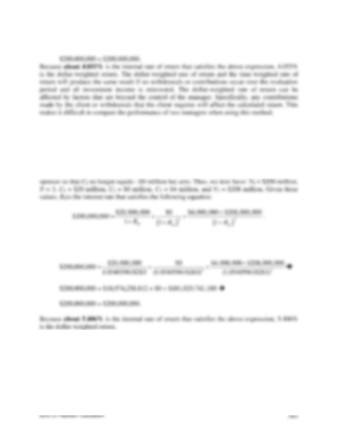
(b) Suppose that the $8 million cash outflow in the second month was a result of withdrawals
by the plan sponsor and that the cash flow after adjusting for this withdrawal is therefore
zero. What would the dollar-weighted rate of return then be for this client’s portfolio?
A cash withdrawal is treated as a cash inflow. So, in the absence of any cash contribution made
by a client for a given time period, a cash withdrawal (e.g., a distribution to a client) is a positive
cash flow for that time period. However, this withdrawal is not by the client but by the plan
( ) ( )
23
111
DDD
RRR
+++
Below we verify that 5.4059618263% or about 5.406% is the internal rate of return satisfies the
above expression.
7. If the average quarterly return for a portfolio is 1.23%, what is the annualized return?
The evaluation period may be less than or greater than one year. Typically, return measures are
reported as an average annual return. This requires the annualization of the subperiod returns.
The subperiod returns are typically calculated for a period of less than one year. The subperiod
returns are then annualized using the following formula:
©2013 Pearson Education
584
annual return = (1 + average period return)number of periods in year – 1.
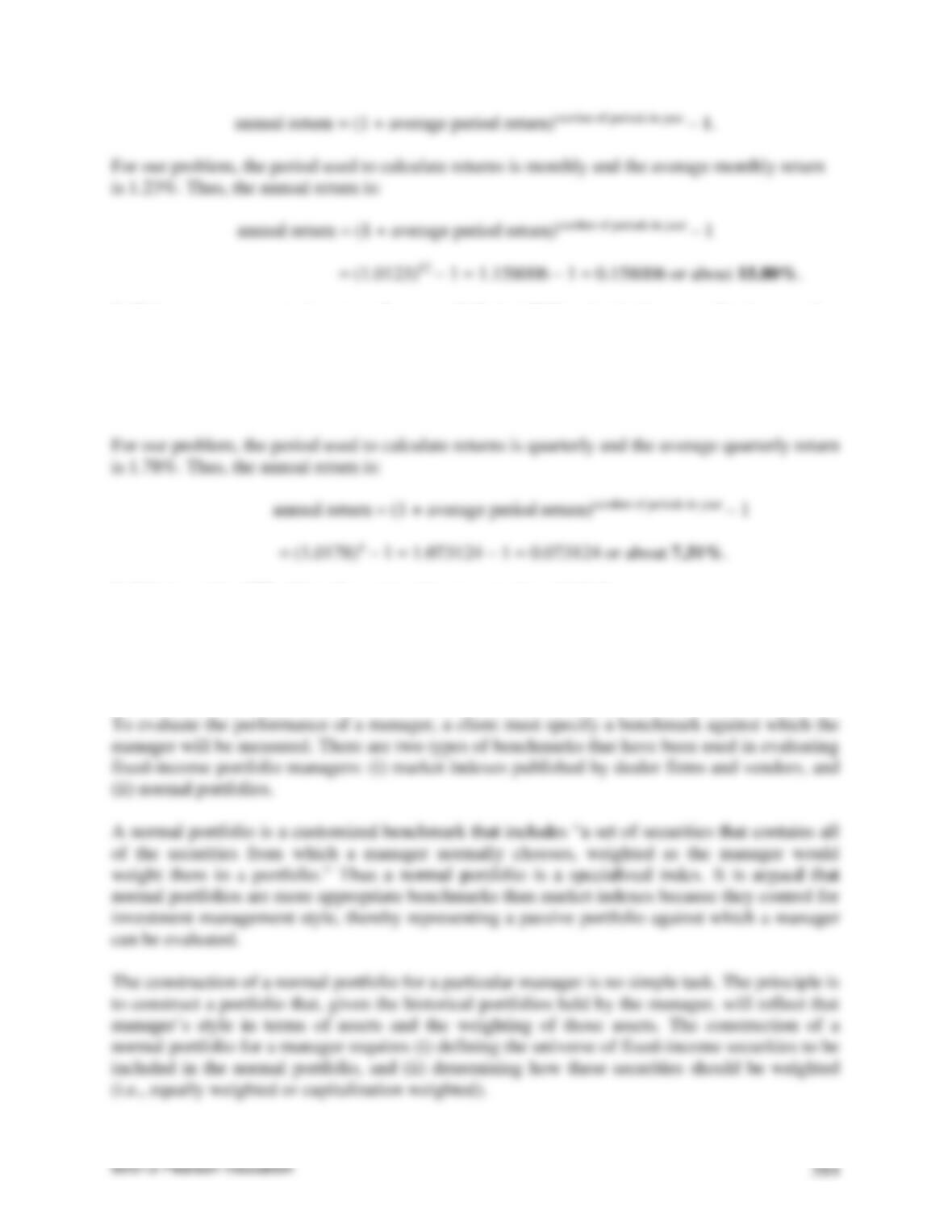
For our problem, the period used to calculate returns is monthly and the average monthly return
is 1.23%. Thus, the annual return is:
annual return = (1 + average period return)number of periods in year – 1
= (1.0123)12 – 1 = 1.158006 – 1 = 0.158006 or about 15.80%.
8. If the average quarterly return for a portfolio is 1.78%, what is the annualized return?
We use the following formula:
annual return = (1 + average period return)number of periods in year – 1.
9. What are the difficulties of constructing a normal portfolio?
The difficulties of constructing a normal portfolio involve defining the universe of fixed-income
securities to be included in the normal portfolio, and determining how these securities should be
weighted. More details are given below.

Defining the set of securities to be included in the normal portfolio begins with discussions
between the client and the manager to determine the manager’s investment style. Based on these
discussions, the universe of all publicly traded securities is reduced to a subset that includes
those securities that the manager considers eligible given his or her investment style.
10. Suppose that the active return for a portfolio over the past year was 130 basis points
after management fees. What questions would you have to before concluding that the
manager’s performance was exceptional?
Clients of asset management firms need to have more information than merely if a portfolio
manager outperformed a benchmark and by how much. For example, you want to know the
reasons. Thus, a first question you might ask is: “What are the reasons for why a portfolio
manager realized the performance relative to the benchmark?” This question is important
because it is possible a pension fund engaged an external manager based on the manager’s claim
that return enhancement can be achieved via security selection.

A third question we might want to ask is: “How did members of the team perform?” Not only do
clients need information about why the portfolio’s return differed from that of the benchmark,
but so do the individuals at the asset management firm engaged by the client. At the firm level,
bonuses to members of the portfolio management team will be determined based on
11. Not only do clients find performance attribution analysis helpful but so does the chief
investment officer of an asset management firm in evaluating the firm’s bond portfolio
team. Explain why.
The chief investment officer of an asset management firm finds it useful for fairly evaluating the
performance of employees and properly allocating bonuses and promotions within the firm.
More details are given below.
At the firm level, bonuses to members of the portfolio management team will be determined
based on performance. Breaking down the performance to the team member level is important
for this purpose, because it impacts decisions about the advancement and retention of such
personnel.
12. A financial institution has hired three external portfolio managers: X, Y, and Z. All three
managers have the same benchmark. A performance attribution analysis of the portfolios
managed by the three managers for the past year was (in basis points):
Risk Factor
Portfolio X
Portfolio Y
Portfolio Z
Yield curve risk
–1
92
–3
Swap spread risk
20
4
20
Volatility risk
40
3
25
Government related spread risk
35
–5
10
Corporate spread risk
–2
6
30
Securitized spread risk
–2
–4
5
The financial institution’s investment committee is using the above information to assess
the performance of the three external managers. Below is a statement from three members
of the performance evaluation committee. Respond to each statement.
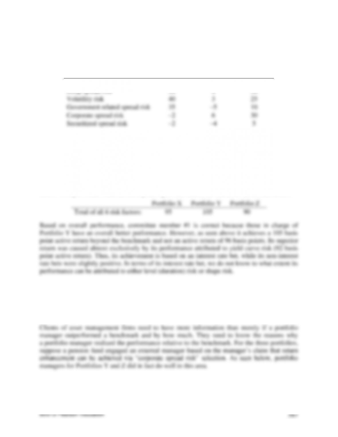
(a) Committee member 1: “Based on overall performance, it is clear that manager Y was the
best performing manager given the 96 basis points.”
Below we report totals when the basis points (plus and minus) are added for all six risk factors:
Portfolio X
Portfolio Y
Portfolio Z
Total of all 6 risk factors:
95
105
90
Based on overall performance, committee member #1 is correct because those in charge of
Portfolio Y have an overall better performance. However, as seen above it achieves a 105 basis
point active return beyond the benchmark and not an active return of 96 basis points. Its superior
return was caused almost exclusively by its performance attributed to yield curve risk (92 basis
point active return). Thus, its achievement is based on an interest rate bet, while its non-interest
rate bets were slightly positive. In terms of its interest rate bet, we do not know to what extent its
performance can be attributed to either level (duration) risk or shape risk.
(b) Committee member 2: “All three of the managers were hired because they claimed that
they had the ability to capitalize on corporate credit opportunities. Although they have all
outperformed the benchmark, I am concerned about the claims that they made when we retained
them.”

©2013 Pearson Education
588
Risk Factor
Portfolio X
Portfolio Y
Portfolio Z
Corporate spread risk
–2
6
30
However, only for Portfolio Z can we say there is strong proof that performance in the corporate
spread risk was achieved. Thus, the concern of committee member #2 is valid due to differences
in performances for the corporate credit products.
(c) Committee member 3: “It seems that managers X and Z were able to outperform the
benchmark without taking on any interest rate risk at all.”
Interest rate risk is captured by the yield curve risk factor, while non-interest rate risk is captured
by the other five risk factors. As seen below, it does appear that committee member #3 is correct
Risk Factor
Portfolio X
Portfolio Y
Portfolio Z
Yield curve risk
–1
92
–3
However, what the above breakdown does not include are the individual components of yield
curve risk (level and shape risks). This is explained in more detail below.
Factor-based attribution models actually allow a decomposition of the yield curve risk into level
(duration) risk and changes in the shape of the yield curve. For example, for the three portfolios
just discussed, suppose that the attribution due to yield curve risk is determined to be as follows:
Risk Factor
Portfolio X
Portfolio Y
Portfolio Z
Yield curve risk
–1
92
–3
Level risk
–51
80
+40
Shape risk
+50
12
–43
Notice that once yield curve risk is decomposed as shown above, it turns out those managers of
Portfolios X and Z did indeed make interest rate bets on both level risk and shape risk. It turns
out that the two bets almost offset each other so there were only small basis point returns
attributable to the interest rate bets. It appears that Portfolio Z’s manager made a major duration
bet and a minor bet on changes in the shape of the yield curve. Thus, as it turns out, committee
member #3 was incorrect as managers of Portfolios X and Z were making greater interest rate
bets than that of Portfolio Y. Thus, given the above breakdown of yield curve risk, their
performance was not all related to their lack of interest rate bets. We one cannot make definitive
conclusions about portfolio managerial performance in terms of interest rate bets without a more
detailed analysis.