Chapter 24 – Portfolio Performance Evaluation
24-1
CHAPTER 24: PORTFOLIO PERFORMANCE EVALUATION
PROBLEM SETS
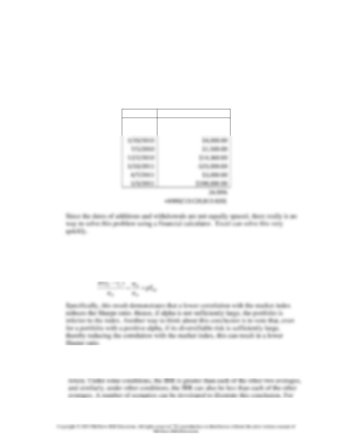
1. The dollar-weighted average will be the internal rate of return between the initial and
final value of the account, including additions and withdrawals. Using Excel’s XIRR
function, utilizing the given dates and values, the dollar-weighted average return is as
follows:
Date
Account
1/1/2010
-$148,000.00
1/3/2010
$2,500.00
$4,000.00
7/5/2010
$1,500.00
4/7/2011
$3,000.00
5/3/2011
2. As established in the following result from the text, the Sharpe ratio depends on both
alpha for the portfolio (
P
) and the correlation between the portfolio and the market
index (ρ):
3. The IRR (i.e., the dollar-weighted return) cannot be ranked relative to either the
geometric average return (i.e., the time-weighted return) or the arithmetic average
Chapter 24 – Portfolio Performance Evaluation
24-2
example, consider a scenario where the rate of return each period consistently
increases over several time periods. If the amount invested also increases each period,
4. It is not necessarily wise to shift resources to timing at the expense of security
5. a. Arithmetic average: ̅rABC = 10%; ̅rXYZ = 10%
c. Geometric average:
rABC = (1.20 × 1.12 × 1.14 × 1.03 × 1.01)1/5 – 1 = 0.0977 = 9.77%
6. a. Time-weighted average returns are based on year-by-year rates of return:
Year
Return = (Capital gains + Dividend)/Price
2013 − 2014
[($120 – $100) + $4]/$100 = 24.00%
Chapter 24 – Portfolio Performance Evaluation
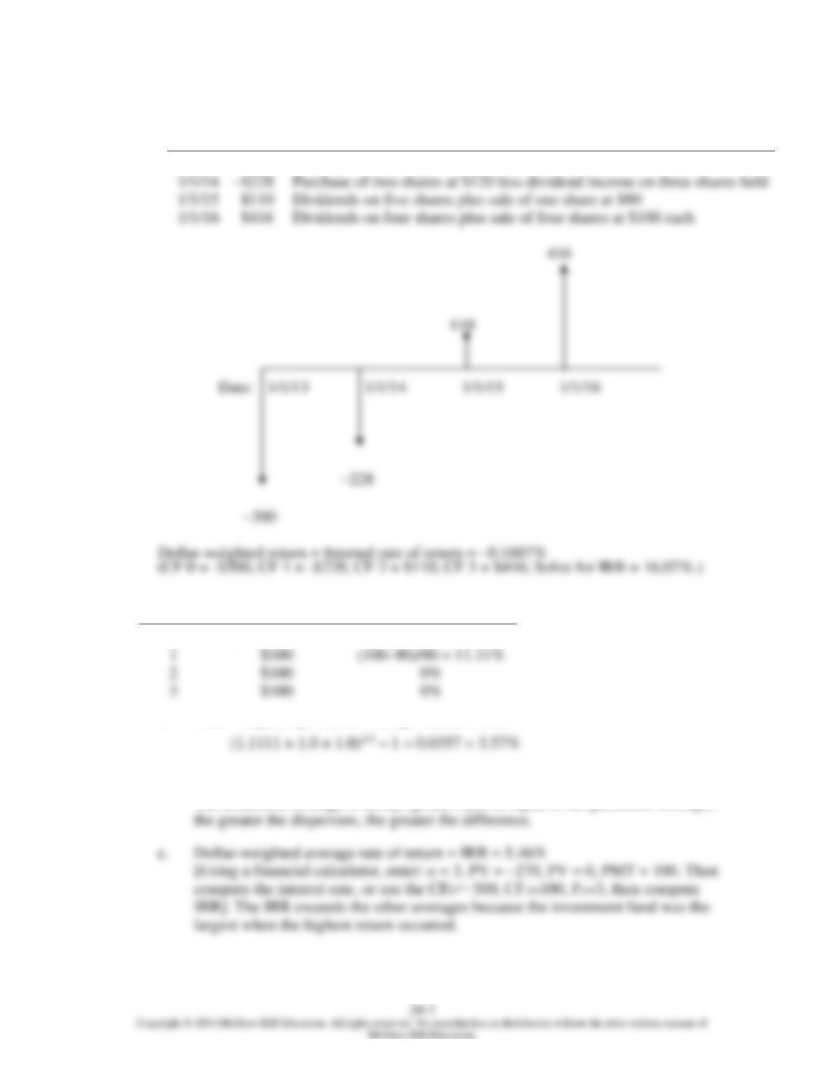
b.
Date
Cash
Flow
Explanation
1/1/13
–$300
Purchase of three shares at $100 each
1/1/14
–$228
Purchase of two shares at $120 less dividend income on three shares held
1/1/15
$110
Dividends on five shares plus sale of one share at $90
1/1/16
$416
Dividends on four shares plus sale of four shares at $100 each
7.
Time
Cash Flow
Holding Period Return
0
3×(–$90) = –$270
1
2
3
a. Time-weighted geometric average rate of return =
b. Time-weighted arithmetic average rate of return = (11.11% + 0 + 0)/3 = 3.70%
The arithmetic average is always greater than or equal to the geometric average;
Chapter 24 – Portfolio Performance Evaluation
24-4
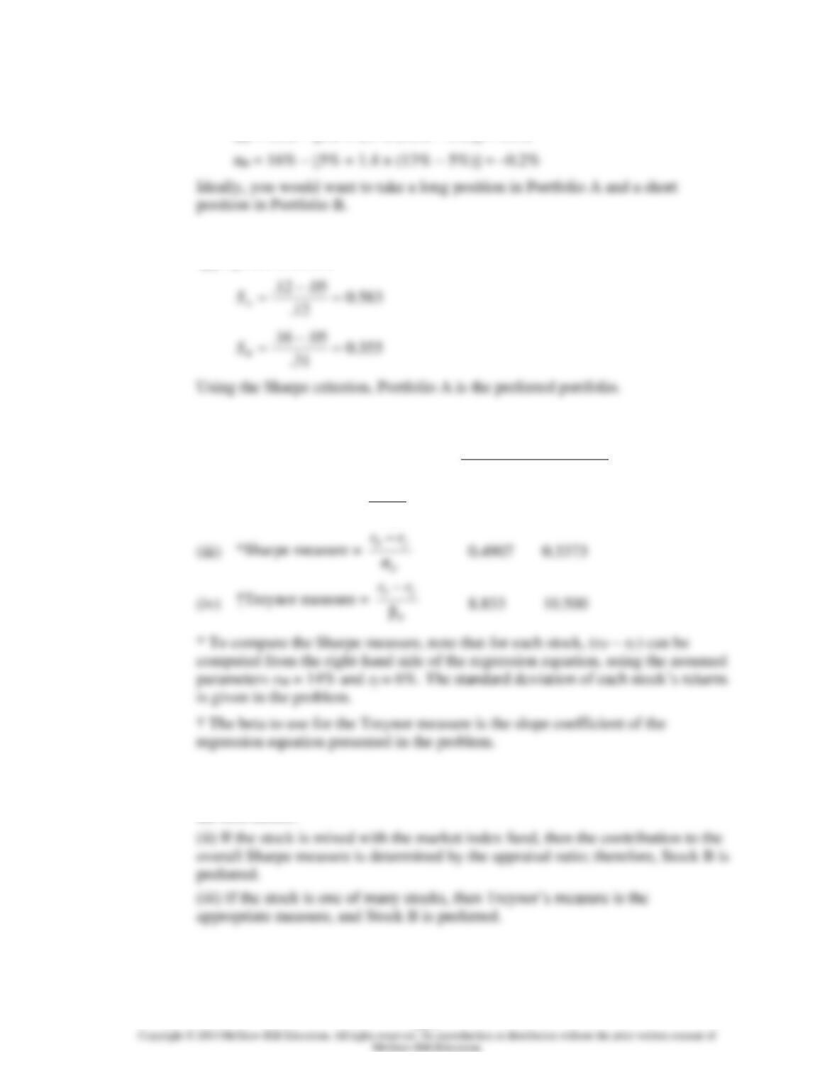
8. a. The alphas for the two portfolios are:
αA = 12% – [5% + 0.7 × (13% – 5%)] = 1.4%
b. If you will hold only one of the two portfolios, then the Sharpe measure is the
appropriate criterion:
9.
a.
Stock A
Stock B
(i)
Alpha = regression intercept
1.0%
2.0%
(ii)
Information ratio =
α
σ(e )
P
P
0.0971
0.1047
b. (i) If this is the only risky asset held by the investor, then Sharpe’s measure is the
appropriate measure. Since the Sharpe measure is higher for Stock A, then A is
the best choice.
Chapter 24 – Portfolio Performance Evaluation
24-5
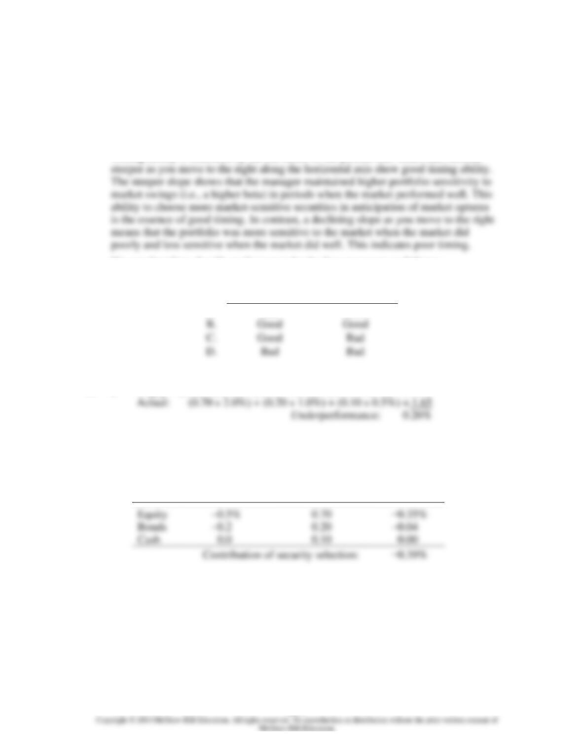
10. We need to distinguish between market timing and security selection abilities.
The intercept of the scatter diagram is a measure of stock selection ability. If the
manager tends to have a positive excess return even when the market’s
performance is merely “neutral” (i.e., has zero excess return), then we conclude
that the manager has on average made good stock picks. Stock selection must be
the source of the positive excess returns.
Timing ability is indicated by the curvature of the plotted line. Lines that become
We can therefore classify performance for the four managers as follows:
Selection
Ability
Timing Ability
A.
Bad
Good
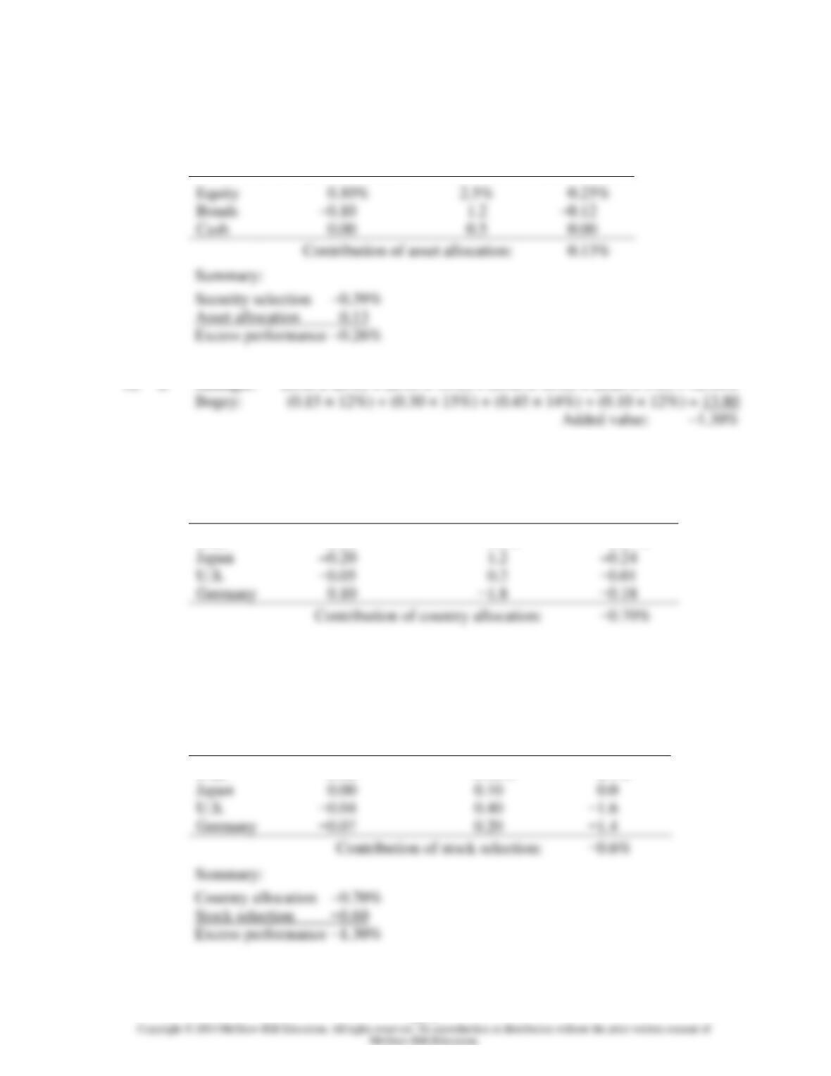
11. a. Bogey: (0.60 × 2.5%) + (0.30 × 1.2%) + (0.10 × 0.5%) = 1.91%
b. Security Selection:
(1)
(2)
(3) = (1) × (2)
Market
Differential Return
within Market
(Manager – Index)
Manager’s
Portfolio
Weight
Contribution to
Performance
0.00
Chapter 24 – Portfolio Performance Evaluation
24-6
c. Asset Allocation:
(1)
(2)
(3) = (1) × (2)
Market
Excess Weight
(Manager – Benchmark)
Index
Return
Contribution to
Performance
Equity
0.25%
Bonds
1.2
Cash
0.5
0.00
0.13%
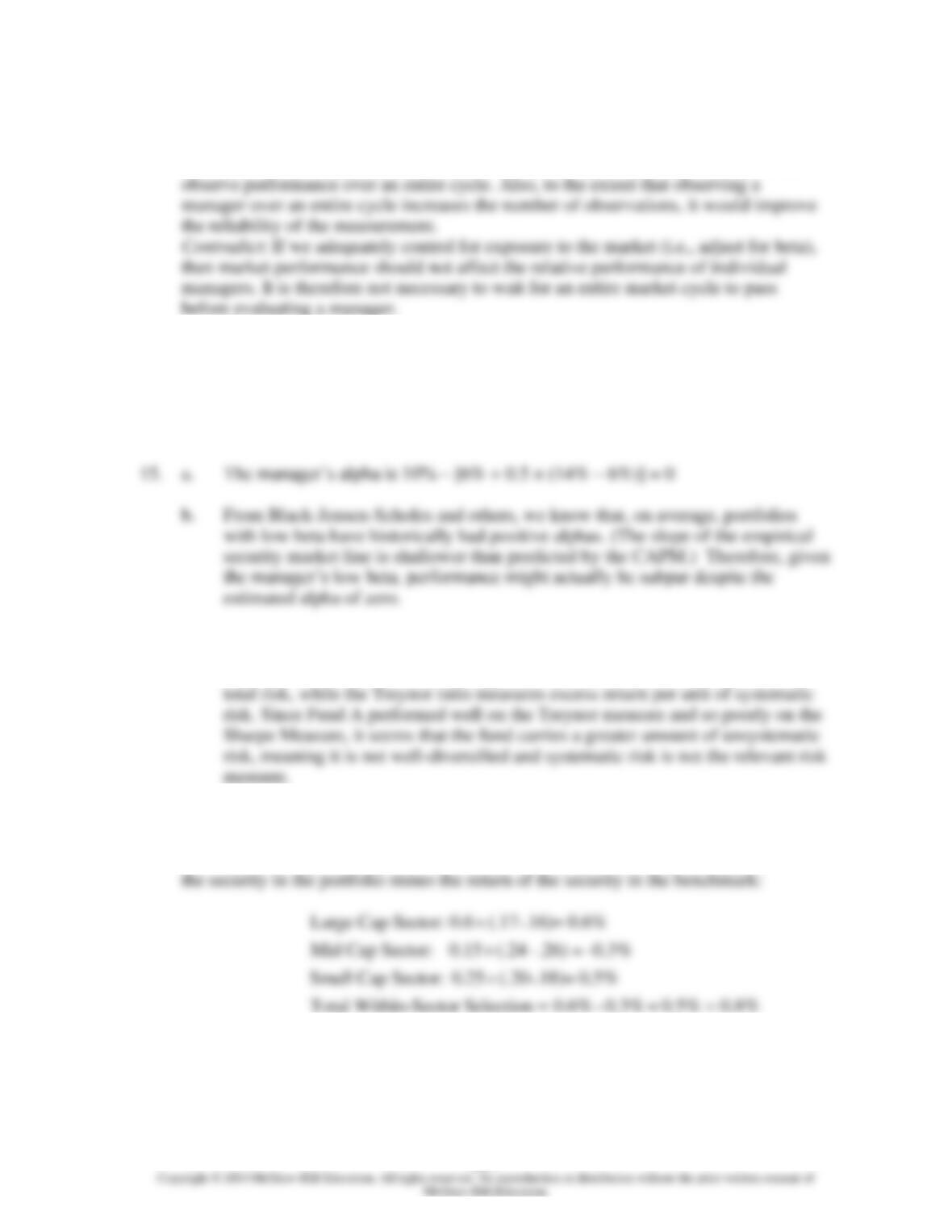
12. a. Manager: (0.30 × 20%) + (0.10 × 15%) + (0.40 × 10%) + (0.20 × 5%) = 12.50%
b. Added value from country allocation:
(1)
(2)
(3) = (1) × (2)
Country
Excess Weight
(Manager – Benchmark)
Index Return
minus Bogey
Contribution to
Performance
U.K.
0.15
−1.8%
−0.27%
Japan
U.S.
−0.01
Germany
0.10
−1.8
−0.18
c. Added value from stock selection:
(1)
(2)
(3) = (1) × (2)
Country
Differential Return
within Country
(Manager – Index)
Manager’s
Country
weight
Contribution to
Performance
U.K.
0.08
0.30%
2.4%
U.S.
0.40
Germany
0.20
Chapter 24 – Portfolio Performance Evaluation
24-7
13. Support: A manager could be a better performer in one type of circumstance than in
another. For example, a manager who does no timing but simply maintains a high
beta, will do better in up markets and worse in down markets. Therefore, we should
14. The use of universes of managers to evaluate relative investment performance does,
to some extent, overcome statistical problems, as long as those manager groups can
be made sufficiently homogeneous with respect to style.
16. a. The most likely reason for a difference in ranking is due to the absence of
diversification in Fund A. The Sharpe ratio measures excess return per unit of
17. The within sector selection calculates the return according to security selection. This is
done by summing the weight of the security in the portfolio multiplied by the return of
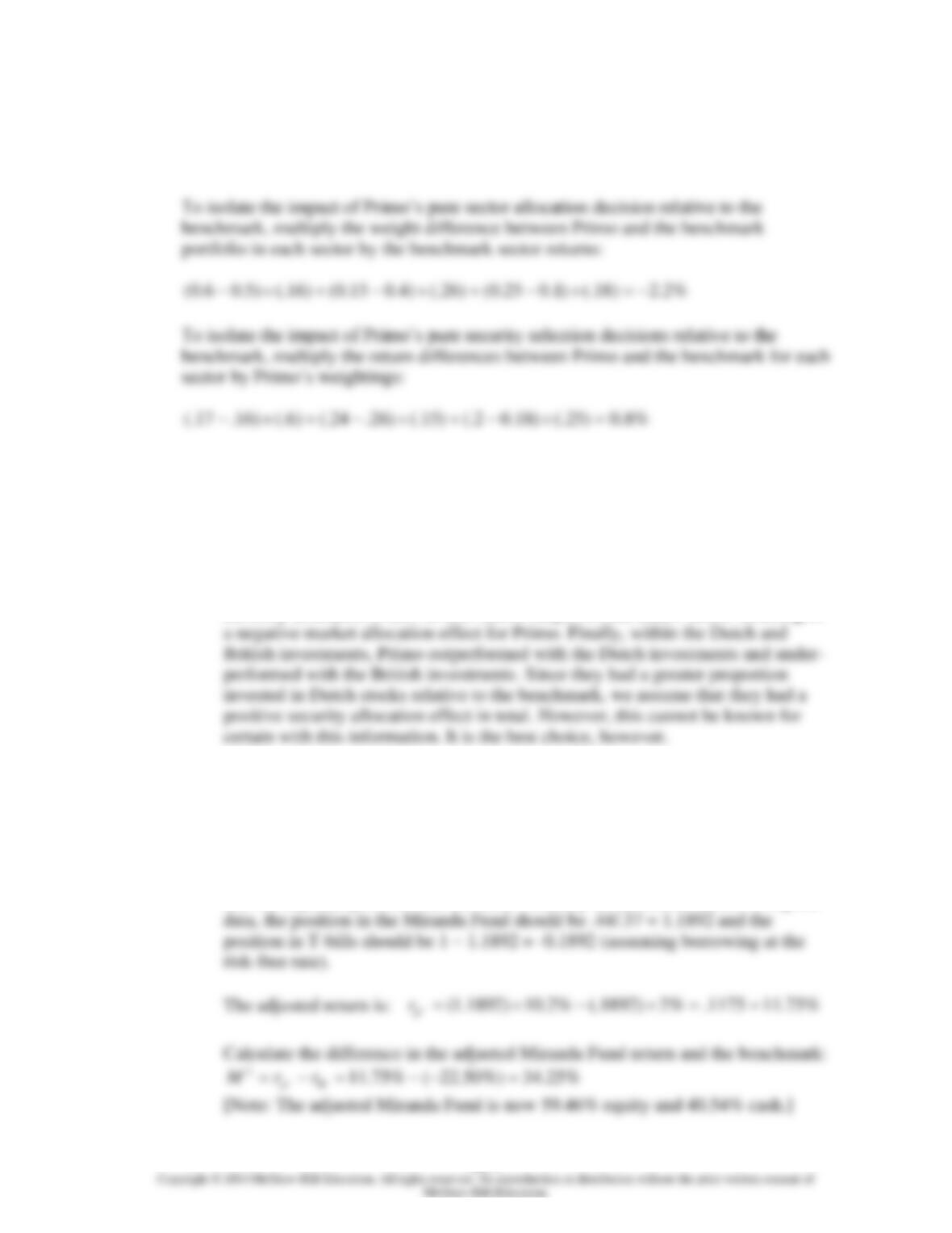
Chapter 24 – Portfolio Performance Evaluation
24-8
18. Primo Return
0.6 17% 0.15 24% 0.25 20% 18.8%= + + =
Benchmark Return
0.5 16% 0.4 26% 0.1 18% 20.2%= + + =
Primo – Benchmark = 18.8% − 20.2% = -1.4% (Primo underperformed benchmark)
19. Because the passively managed fund is mimicking the benchmark, the
2
R
of the
regression should be very high (and thus probably higher than the actively managed
fund).
20. a. The euro appreciated while the pound depreciated. Primo had a greater stake in
the euro-denominated assets relative to the benchmark, resulting in a positive
currency allocation effect. British stocks outperformed Dutch stocks resulting in
21. a.
Miranda S&P
.102 .02 .225 .02
.2216 .5568
σ .37 .44
Pf
P
rr SS
−− − −
→ = = = =
b. To compute
2
M
measure, blend the Miranda Fund with a position in T-bills such
that the adjusted portfolio has the same volatility as the market index. Using the

Chapter 24 – Portfolio Performance Evaluation
c.
Miranda S&P
.102 .02 .225 .02
.0745 .245
β 1.10 1.00
Pf
P
rr TT
−− − −
→ = = = = −
22. This exercise is left to the student; answers will vary.
CFA PROBLEMS
1. a. Manager A
Strength. Although Manager A’s one-year total return was somewhat below the
international index return (–6.0 percent versus –5.0 percent), this manager
Manager B
Strength. Manager B’s total return exceeded that of the index, with a marked
positive increment apparent in the currency return. Manager B had a –1.0 percent
b. The following strategies would enable the fund to take advantage of the
strengths of each of the two managers while minimizing their weaknesses.
1. Recommendation: One strategy would be to direct Manager A to make
no currency bets relative to the international index and to direct Manager
B to make only currency decisions, and no active country or security
Chapter 24 – Portfolio Performance Evaluation
24–10
2. Recommendation: Another strategy would be to combine the portfolios of
Manager A and Manager B, with Manager A making country exposure and
2. a. Indeed, the one year results were terrible, but one year is a poor statistical base
from which to draw inferences. Moreover, the board of trustees had directed Karl
to adopt a long-term horizon. The board specifically instructed the investment
manager to give priority to long-term results.
b. The sample of pension funds had a much larger share invested in equities than
bad for bonds, the asset class that Alpine had been encouraged to hold. Within
this asset class, however, Alpine did much better than the index fund.
Moreover, despite the fact that the bond index underperformed both the
3. a. Method I does nothing to separately identify the effects of market timing and
security selection decisions. It also uses a questionable “neutral position,” the
composition of the portfolio at the beginning of the year.
b. Method II is not perfect but is the best of the three techniques. It at least attempts

Chapter 24 – Portfolio Performance Evaluation
24–11
c. Method III uses net purchases of bonds as a signal of bond manager optimism.
4. Treynor measure =
17 8 8.182
1.1
−=
5. Sharpe measure =
(.24 .08) 0.888
.18
−=
6. a. Treynor measures
(10 6) (12 6)
Portfolio X: 6.67 S&P 500: 6.00
0.6 1.0
−−
==
7. Geometric average = (1.15 × 0.90)1/2 – 1 = 0.0173 = 1.73%
10. d.
Chapter 24 – Portfolio Performance Evaluation
24–12
CF0 = −$500,000
12. a. Each of these benchmarks has several deficiencies, as described below.
Market index:
• A market index may exhibit survivorship bias. Firms that have gone out of
business are removed from the index, resulting in a performance measure that
overstates actual performance had the failed firms been included.
• A market index may exhibit double counting that arises because of companies
owning other companies and both being represented in the index.
Benchmark normal portfolio:
• This is the most difficult performance measurement method to develop and
calculate.
Median of the manager universe:
• It can be difficult to identify a universe of managers appropriate for the
investment style of the plan’s managers.
• Selection of a manager universe for comparison involves some, perhaps much,
Chapter 24 – Portfolio Performance Evaluation
24–13
• The benchmark is not constructed prior to the start of an evaluation period; it is
not specified in advance.
b. i. The Sharpe ratio is calculated by dividing the portfolio risk premium (i.e.,
actual portfolio return minus the risk-free return) by the portfolio standard
deviation:
Sharpe ratio =
β
Pf
rr−
σ
Pf
rr−
ii. The Sharpe ratio assumes that the relevant risk is total risk, and it measures
excess return per unit of total risk. The Treynor measure assumes that the
relevant risk is systematic risk, and it measures excess return per unit of
systematic risk. Jensen’s alpha assumes that the relevant risk is systematic
risk, and it measures excess return at a given level of systematic risk.
13. i. Incorrect. Valid benchmarks are unbiased. Median manager benchmarks,
however, are subject to significant survivorship bias, which results in several
drawbacks, including the following:
• The performance of median manager benchmarks is biased upwards.
ii. Incorrect. Valid benchmarks are unambiguous and can be replicated. The median
manager benchmark is ambiguous because the weights of the individual
Chapter 24 – Portfolio Performance Evaluation
24–14
14. a. Sharpe ratio =
β
Pf
rr−
σ
Pf
rr−
b. The difference in the rankings of Williamson and Joyner results directly from the
difference in diversification of the portfolios. Joyner has a higher Treynor