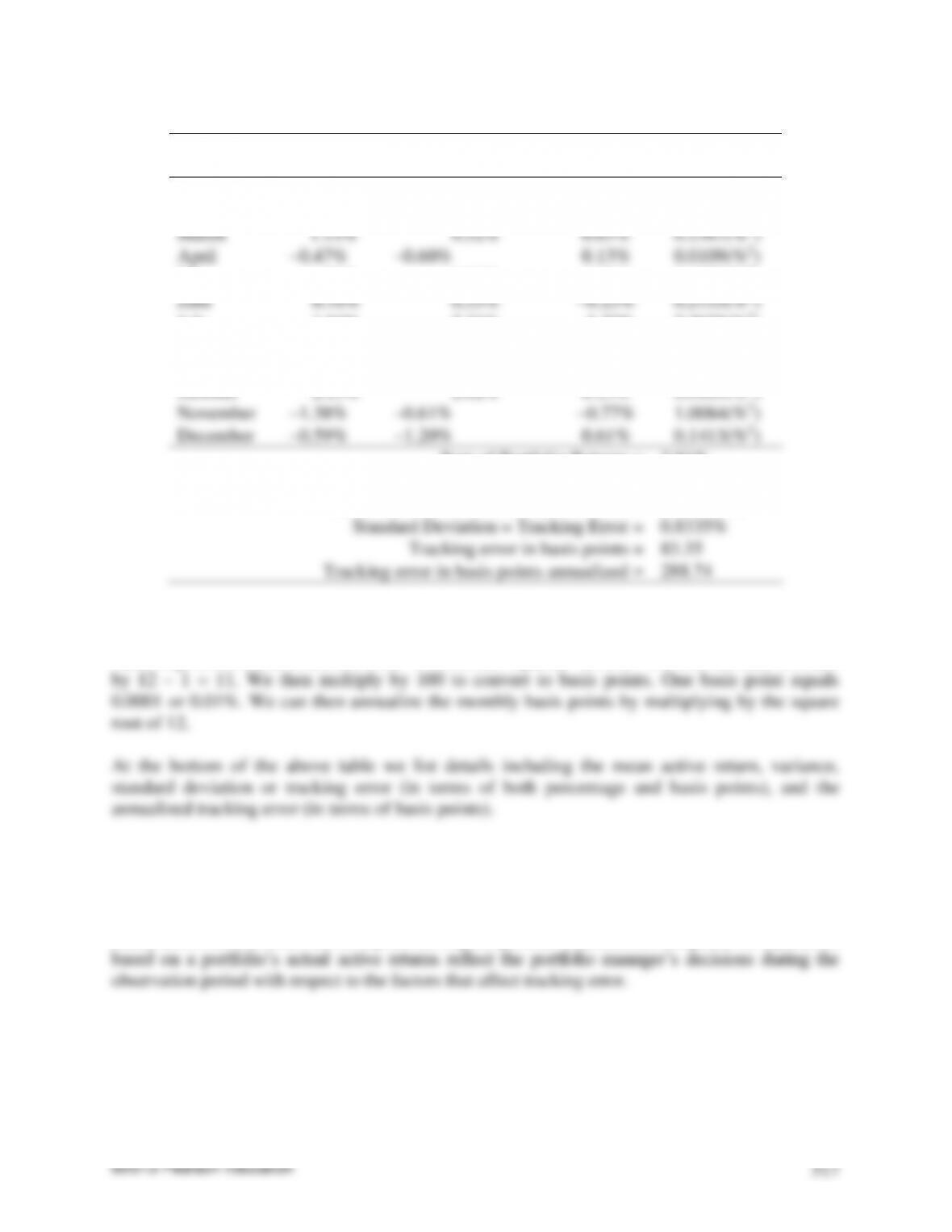
Month 2001
Portfolio
A’s Return
Lehman Aggregate
Bond Index Return
Active
Return
Differences
Squared
January
2.15%
1.65%
0.50%
0.0707(%2)
February
0.89%
–0.10%
0.99%
0.5713(%2)
March
1.15%
0.52%
0.63%
0.1567(%2)
April
–0.47%
–0.60%
0.13%
0.0109(%2)
May
1.71%
0.65%
1.06%
0.6820(%2)
June
0.10%
0.33%
–0.23%
0.2155(%2)
July
1.04%
2.31%
–1.27%
2.2625(%2)
August
2.70%
1.10%
1.60%
1.8655(%2)
September
0.66%
1.23%
–0.57%
0.6467(%2)
October
2.15%
2.02%
0.13%
0.0109(%2)
November
–1.38%
–0.61%
–0.77%
1.0084(%2)
December
–0.59%
–1.20%
0.61%
0.1413(%2)
Sum of Portfolio Returns =
2.81%
Mean Active Return =
0.2342%
Variance (sum of differences squared / 11) =
0.6947(%2)
Standard Deviation = Tracking Error =
0.8335%
Tracking error in basis points =
83.35
Tracking error in basis points annualized =
288.74
To compute the standard deviation of these active returns, we subtract the average (or mean)
active return from each active return, and then square each difference. Each difference squared
value is given in the table above in the “Differences Squared” column. We then divided this sum
(b) Is the tracking error computed in part (a) a backward-looking or forward-looking
tracking error?
The tracking error computed in part (a) is backward-looking because it is calculated based on the
actual active returns observed for a portfolio is prior periods. Calculations computed for a portfolio
(c) Compare the tracking error found in part (a) to the tracking error found for Portfolios
A and B in Exhibits 23-1 and 23-2. What can you say about the investment management
strategy pursued by this portfolio manager?
The tracking error found for our problem is greater especially compared to Portfolio A. A greater

©2013 Pearson Education
518
tracking error means greater deviation from the benchmark. This is seen if we compare active
return values from our table with the greater active return values found in the exhibits. For our
problem, it appears the manager may be employing a high-risk strategy to enhance the indexed
portfolio’s return. This strategy is commonly referred to as enhanced indexing or indexing
plus.
11. Assume the following:
benchmark index = Salomon Smith Barney BIG Bond Index
Assuming that returns are normally distributed, complete the following table:
Number of Standard
Deviations
Range for Portfolio
Active Return
Corresponding Range
for Portfolio Return
Probability
1
2
3
With an expected return of 7% and a standard deviation of 200 basis points or 2%, then a normal
distribution implies there is about a 67% probability that values will be found between one
standard deviation of either side of the mean. Thus, for a standard deviation of 1, the range on
either side of the mean for portfolio active return is 1 standard deviation times 2% = 2%. The 2%
Likewise, for a standard deviation of three, the range on either side of the mean is 3 standard
deviation times 2% = 6%. With a portfolio mean active return of 7%, the corresponding range
The above values can all be found in the below table.
Number of Standard
Deviations
Range for Portfolio
Active Return
Corresponding Range
for Portfolio Return
Probability
1
2%
5%–9%
67%
2
4%
3%–11%
95%

3
6%
1%–13%
99%
12. At a meeting between a portfolio manager and a prospective client, the portfolio manager
stated that her firm’s bond investment strategy is a conservative one. The portfolio manager
told the prospective client that she constructs a portfolio with a forward-looking tracking
error that is typically between 250 and 300 basis points of a client-specified bond index.
Explain why you agree or disagree with the portfolio manager’s statement that the portfolio
strategy is a conservative one.
If the chosen benchmark is the desired norm, then greater deviation from the norm implies more
risk taking, i.e., less conservative than claimed by the portfolio manager. Regardless, it appears
the manager is pursuing an active strategy that involves risk taking. More details are given
below.
Second, the strategy is not passive. When a portfolio is constructed to have a forward-looking
tracking error of zero, the manager has effectively designed the portfolio to replicate the
performance of the benchmark. If the forward-looking tracking error is maintained for the entire
13. What is meant by tracking error due to systematic risk factors?
By tracking error due to systematic risk factors, we mean tracking error caused by factors that
affect the return of securities in the benchmark in varying degrees. More details are given below.
Forward-looking tracking error indicates the degree of active portfolio management being
pursued by a manager. Therefore, it is necessary to understand what factors (including
systematic risk factors) affect the performance of a manager’s benchmark index. The degree to
which the manager constructs a portfolio that has exposure to the risk factors that is different
from the risk factors that affect the benchmark determines the forward-looking tracking error.
14. You are reviewing a report by a portfolio manager that indicates that a fund’s predicted
(forward-looking) tracking error is 94.87 basis points. Furthermore, it is reported that the
predicted tracking error due to systematic risk is 90 basis points and the predicted tracking
error due to non-systematic risk is 30 basis points. Why doesn’t the sum of these two
tracking error components total up to 94.87 basis points?
The predicted tracking error is 94.87 basis points. The two major risk categories are systematic
and non-systematic risks. For our portfolio, they are respectively 90 basis points and 30 basis
points. Now this might seem confusing since adding these two risks we do not get to the
predicted tracking error of 94.87 basis points for the portfolio. The reason is that these risk
15. What are the drawbacks of the cell-based approach for bond portfolio construction?

Let us first describe the cell-based approach. Under the cell-based approach, the benchmark is
divided into cells, each cell representing a different characteristic of the benchmark. The most
common cells used to break down a benchmark are (1) duration, (2) coupon, (3) maturity,
(4) market sectors, (5) credit quality, (6) call factors, and (7) sinking fund features.
The number of cells that the indexer uses will depend on the dollar amount of the portfolio. In
a portfolio of less than $100 million, for example, using a large number of cells entails
a problem. The “drawback” faced by the manager is it would require purchasing odd lots of
issues. This increases the cost of buying the issues to represent a cell and thus would increase the
16. Why is it difficult to build a portfolio in pursuing a pure bond indexing strategy?
While it is not simple to build a portfolio for enhanced indexing strategies, it is even more
difficult to implement a pure bond indexing strategy. These grave difficulties apply to both the
cell-based and multi-factor model approaches to portfolio construction. Below we attempt to
describe why.
In a pure bond indexing strategy, the portfolio manager must purchase all of the issues in the
bond index according to their weight in the benchmark index. However, substantial tracking
error will result from the transaction costs (and other fees) associated with purchasing all the
issues and reinvesting cash flow (maturing principal and coupon interest). A broad-based market

forced to follow an enhanced bond indexing strategy with minor mismatches in the primary risk
factors.
A portfolio manager faces several other logistical problems in seeking to construct an indexed
portfolio. First, the prices for each issue used by the organization that publishes the index may
not be execution prices available to the indexer. In fact, they may be materially different from the
prices offered by some dealers. In addition, the prices used by organizations reporting the value
of indexes are based on bid prices. Dealer ask prices, however, are the ones that the manager
17. How can a multi-factor risk model be used to monitor and control portfolio risk?
A multi-factor risk model can be used to monitor and control portfolio risk through
a forward-looking estimate of tracking error. The portfolio manager needs this forward-looking
estimate of tracking error to reflect the portfolio risk going forward. The way this is done in
practice is by using the services of a commercial vendor or dealer firm that has modeled the
factors that affect the tracking error associated with the bond market index (i.e., the portfolio
From the properties of a normal distribution, we know the following:
Number of Standard
Deviations
Range for Portfolio
Active Return
Corresponding Range for
Portfolio Return
Probability
1
–1%
9%–11%
67%
2
–2%
8%–12%
95%
3
–3%
7%–13%
99%
The forward-looking tracking error is useful in risk control and portfolio construction. The
manager can immediately see the likely effect on tracking error of any intended change in the
portfolio. Thus, scenario analysis can be performed by a portfolio manager to assess proposed
portfolio strategies and eliminate those that would result in tracking error beyond a specified
tolerance for risk.
18. How can a multi-factor risk model be used to rebalance a portfolio?
While it is common to illustrate portfolio construction starting with a position of cash and
building a portfolio of securities, in practice the more common task is to rebalance an existing
portfolio. A multi-factor model along with an optimizer can be used to efficiently rebalance the
portfolio. This rebalancing using a multi-factor model involves realigning the portfolio that has
optimizer can identify a package of transactions (i.e., sells and buys) and identify the reduction
(or increase) in risk that would result from the execution of those transactions so that the
portfolio manager can assess the risk adjustment benefit relative to the cost of executing the
transaction.
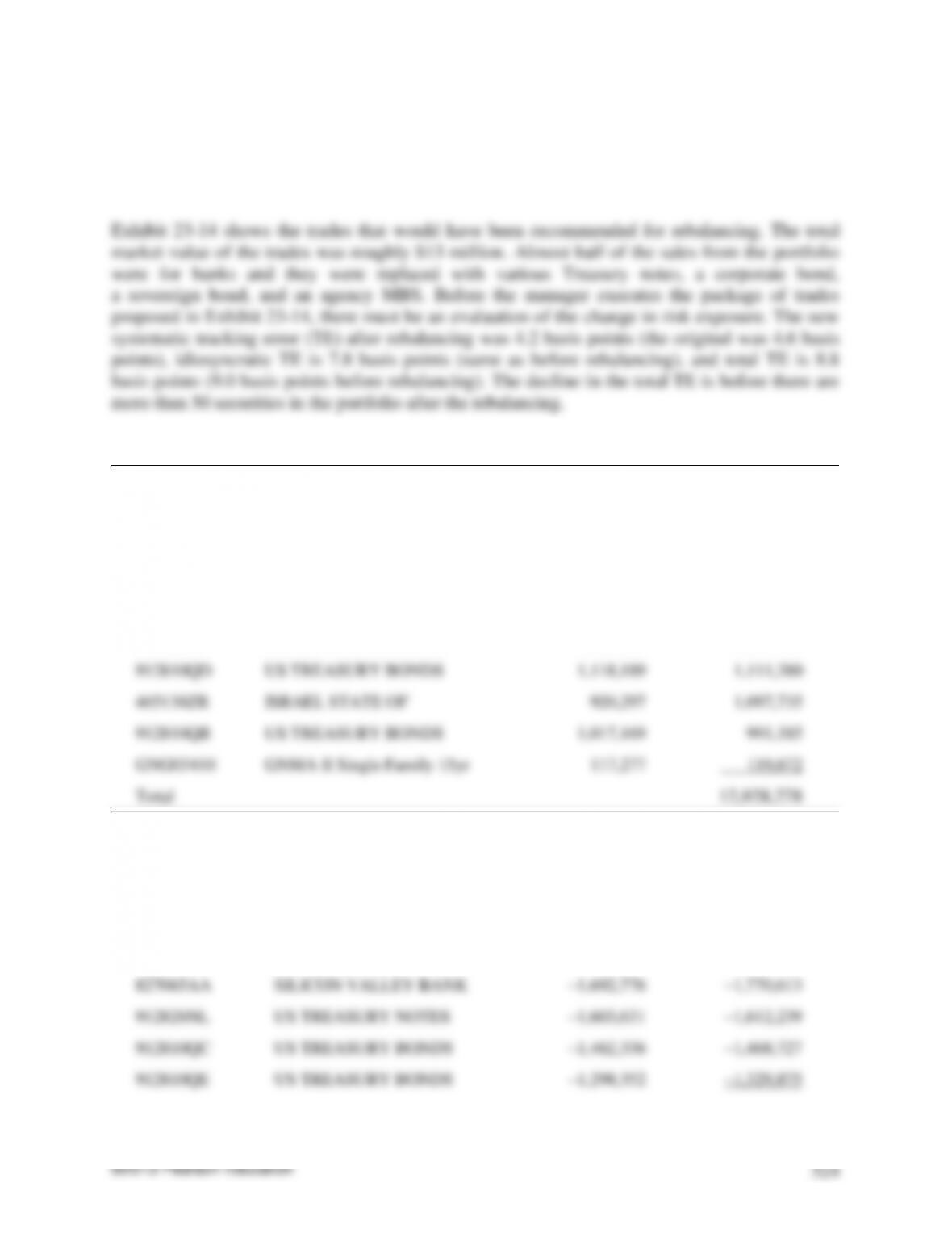
Exhibit 23-14Trades for Portfolio Rebalancing
Buys
Identifier
Description
Position Amount
Market Value
912828LK
US TREASURY NOTES
3,133,909
3,235,179
912828LS
US TREASURY NOTES
2,814,967
2,924,353
489170AB
KENNAMETAL INC
1,959,720
2,087,886
94986EAA
WELLS FARGO CAPITAL XIII
1,286,097
1,360,888
912810QD
US TREASURY BONDS
1,118,189
1,111,380
465138ZR
ISRAEL STATE OF
920,297
1,097,735
912810QB
US TREASURY BONDS
1,017,169
991,185
GNG03410
GNMA II Single Family 15yr
117,277
119,672
Total
12,928,278
Sells
Identifier
Description
Position Amount
Market Value
912828NV
US TREASURY NOTES
–2,662,260
–2,586,183
16132NAV
CHARTER ONE BANK FSB
–2,203,358
–2,332,312
05946NAD
BANCO BRADESCO SA
–1,564,870
–1,828,328
827065AA
SILICON VALLEY BANK
–1,692,776
–1,770,613
912828NL
US TREASURY NOTES
–1,603,631
–1,612,239
912810QC
US TREASURY BONDS
–1,462,336
–1,468,727
912810QE
US TREASURY BONDS
–1,298,352
–1,329,875

Total
–12,928,278
19. In a factor model, what is meant by isolated tracking error?
An isolated tracking error refers to the method of calculating the partial tracking error due to
a single group of risk factors in isolation; no other forms of risk are considered. Illustrations
giving more details are given below.
Let us first illustrate an isolated tracking error by considering the risk factor “securitized spread”
in Exhibit 23-7. This risk factor is the exposure to changes in the spreads in the agency MBS
market. The value of 2.5 means that if the portfolio only differs from the benchmark with respect
to its exposure to changes in the spread in the agency MBS sector, then this mismatch relative to
the benchmark would result in a monthly isolated tracking error of 2.5 basis points.
Portfolio isolated systematic TE = [(TE1)2 + (TE2)2 + … + (TEK)2]1/2
where TE denotes tracking error and the subscript denotes the risk factor.
Consider the 50-security portfolio in Exhibit 23-13 where the monthly isolated TE for each risk
factor is shown in Exhibit 23-7. Here the portfolio isolated systematic TE is 6.24 basis points per
month as shown below:
©2013 Pearson Education
526
Portfolio TE = [(TEF1)2 + (TEF2)2 + 2 Cov(F1,F2)]1/2
where Cov(F1,F2) is the covariance between risk factor exposures 1 and 2.
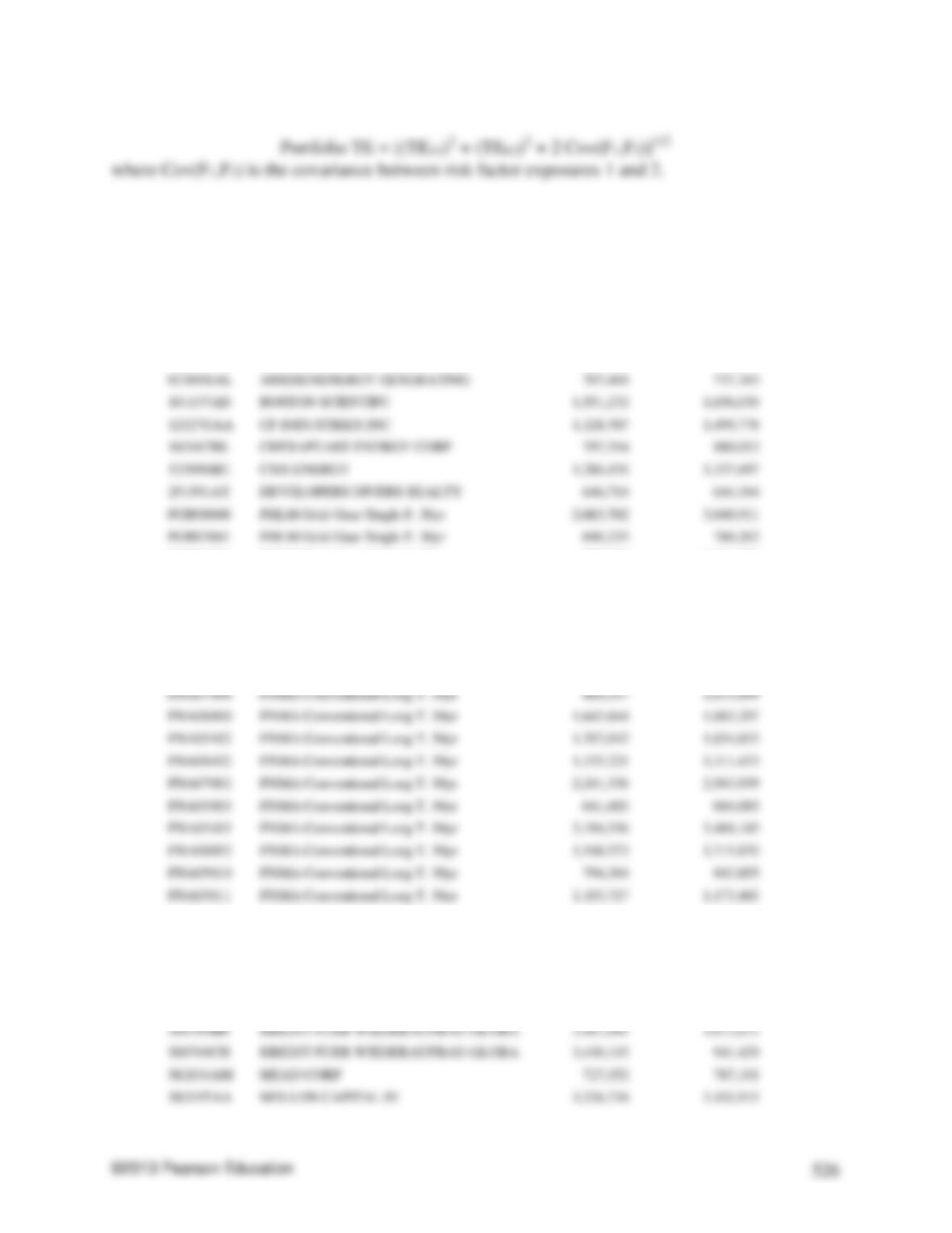
20. Following is a portfolio consisting of 50 bonds with a market value of $100 million as of
April 29, 2011:
Identifier
Description
Position
Market Value
003723AA
ABN AMRO BANK NV
1,449,636
1,422,596
00104BAC
AES EASTERN ENERGY
1,682,044
1,206,446
02051PAC
ALON REFINING KROTZ
592,304
630,655
02360XAL
AMERENENERGY GENERATING
707,484
737,343
101137AD
BOSTON SCIENTIFC
1,551,232
1,656,030
12527GAA
CF INDUSTRIES INC
1,328,707
1,499,778
165167BS
CHESAPEAKE ENERGY CORP
797,314
880,013
125896BG
CMS ENERGY
1,286,476
1,337,697
251591AY
DEVELOPERS DIVERS REALTY
646,714
644,344
FGB08000
FHLM Gold Guar Single F. 30yr
2,683,702
3,040,911
FGB07001
FHLM Gold Guar Single F. 30yr
690,235
780,262
FGB06402
FHLM Gold Guar Single F. 30yr
885,600
1,004,579
FGB07002
FHLM Gold Guar Single F. 30yr
3,751,831
4,235,068
FGB05403
FHLM Gold Guar Single F. 30yr
1,411,009
1,531,707
FGB06003
FHLM Gold Guar Single F. 30yr
1,387,727
1,537,027
FGB06004
FHLM Gold Guar Single F. 30yr
633,691
700,545
FGB05011
FHLM Gold Guar Single F. 30yr
651,568
690,585
FNA07098
FNMA Conventional Long T. 30yr
884,357
1,014,899
FNA08000
FNMA Conventional Long T. 30yr
1,643,844
1,883,297
FNA05402
FNMA Conventional Long T. 30yr
1,707,042
1,854,853
FNA06402
FNMA Conventional Long T. 30yr
1,155,221
1,311,433
FNA07002
FNMA Conventional Long T. 30yr
2,241,336
2,563,939
FNA05003
FNMA Conventional Long T. 30yr
641,485
684,085
FNA05403
FNMA Conventional Long T. 30yr
3,194,556
3,469,103
FNA06003
FNMA Conventional Long T. 30yr
1,548,573
1,715,870
FNA05010
FNMA Conventional Long T. 30yr
794,384
843,855
FNA05011
FNMA Conventional Long T. 30yr
1,105,717
1,173,465
GNB04411
GNMA II Single Family 30yr
2,391,899
2,509,580
381427AA
GOLDMAN SACHS CAPITAL II
3,123,435
2,761,546
45905CAA
INTERNATL BANK RECON DEV-GLOBA
1,151,247
1,200,080
45950KBJ
INTL FINANCE CORPORATION
1,227,607
1,198,808
46513E5Y
ISRAEL STATE OF-GLOBAL
1,797,220
1,911,761
500769BR
KREDIT FUER WIEDERAUFBAU-GLOBA
3,461,061
1,012,672
500769CH
KREDIT FUER WIEDERAUFBAU-GLOBA
3,430,115
941,429
582834AM
MEAD CORP
727,352
787,191
58551TAA
MELLON CAPITAL IV
3,326,734
3,102,915
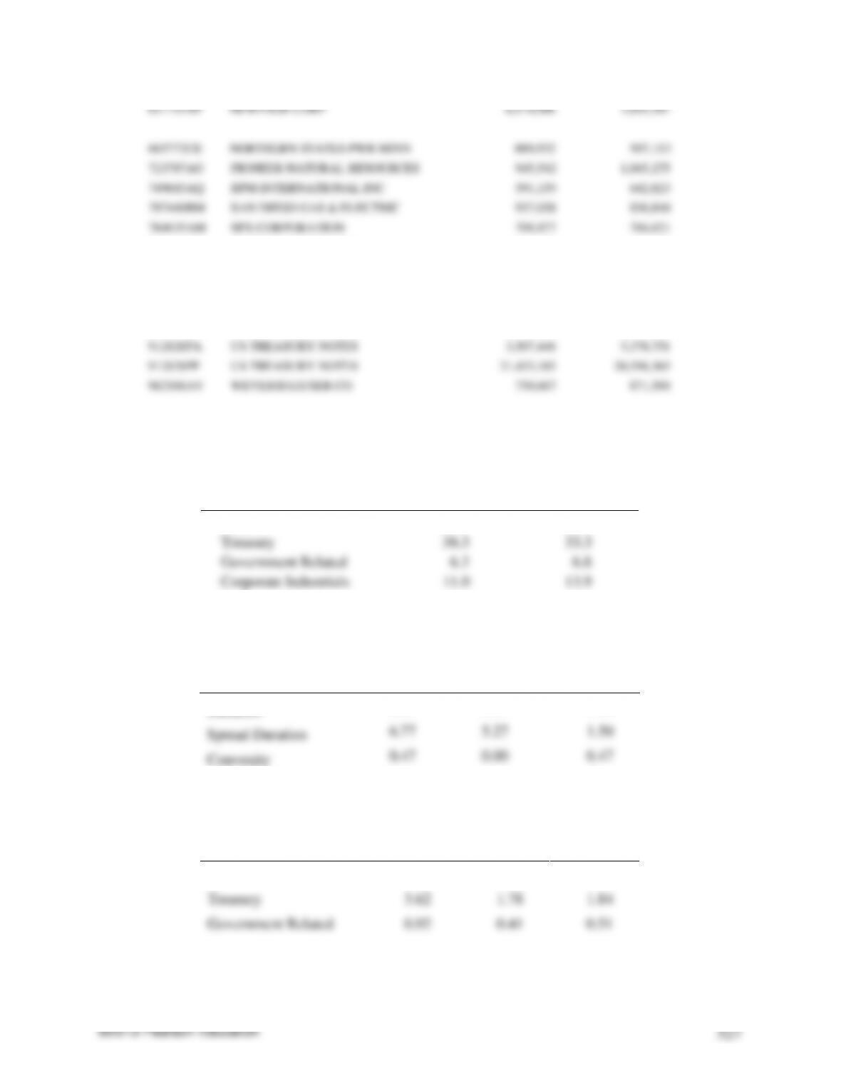
651715AF
NEWPAGE CORP
6,414,006
1,603,501
665772CE
NORTHERN STATES PWR MINN
889,932
907,113
723787AG
PIONEER NATURAL RESOURCES
945,542
1,045,275
749685AQ
RPM INTERNATIONAL INC
591,159
642,823
797440BM
SAN DIEGO GAS & ELECTRIC
957,058
856,840
784635AM
SPX CORPORATION
708,877
766,621
91311QAD
UNITED UTILITES PLC
844,170
848,272
915436AF
UPM-KYMMENE CORP
655,540
648,265
912810PW
US TREASURY BONDS
797,859
804,588
912810QA
US TREASURY BONDS
8,725,929
7,505,533
912810QK
US TREASURY BONDS
4,408,259
4,048,097
912828PA
US TREASURY NOTES
3,507,446
3,378,751
912828PF
US TREASURY NOTES
21,453,185
20,596,365
962166AV
WEYERHAEUSER CO
750,667
871,588
The benchmark for the manager who has constructed this portfolio is a composite index
consisting one-third each of the Barclays Capital U.S. Treasury index, Barclays Capital U.S.
Credit Index, and Barclays Capital U.S. MBS index.
Asset Class
Portfolio
Benchmark
Total
100.0
100.0
Treasury
36.3
33.3
Government Related
6.3
6.8
Corporate Industrials
11.0
13.9
Corporate Utilities
5.9
2.9
Corporate Financials
7.9
9.7
MBS Agency
32.6
33.3
Analytics
Portfolio
Benchmark
Difference
Duration
6.87
5.37
1.50
Spread Duration
6.77
5.27
1.50
Convexity
0.47
0.00
0.47
Vega
0.01
0.03
0.02
Spread
355
55
300.00
Duration Contribution
Portfolio
Benchmark
Difference
Total
6.87
5.37
1.50
Treasury
3.62
1.78
1.84
Government Related
0.92
0.41
0.51
Corporate
1.10
1.74
–0.63
Securitized
1.23
1.45
–0.22
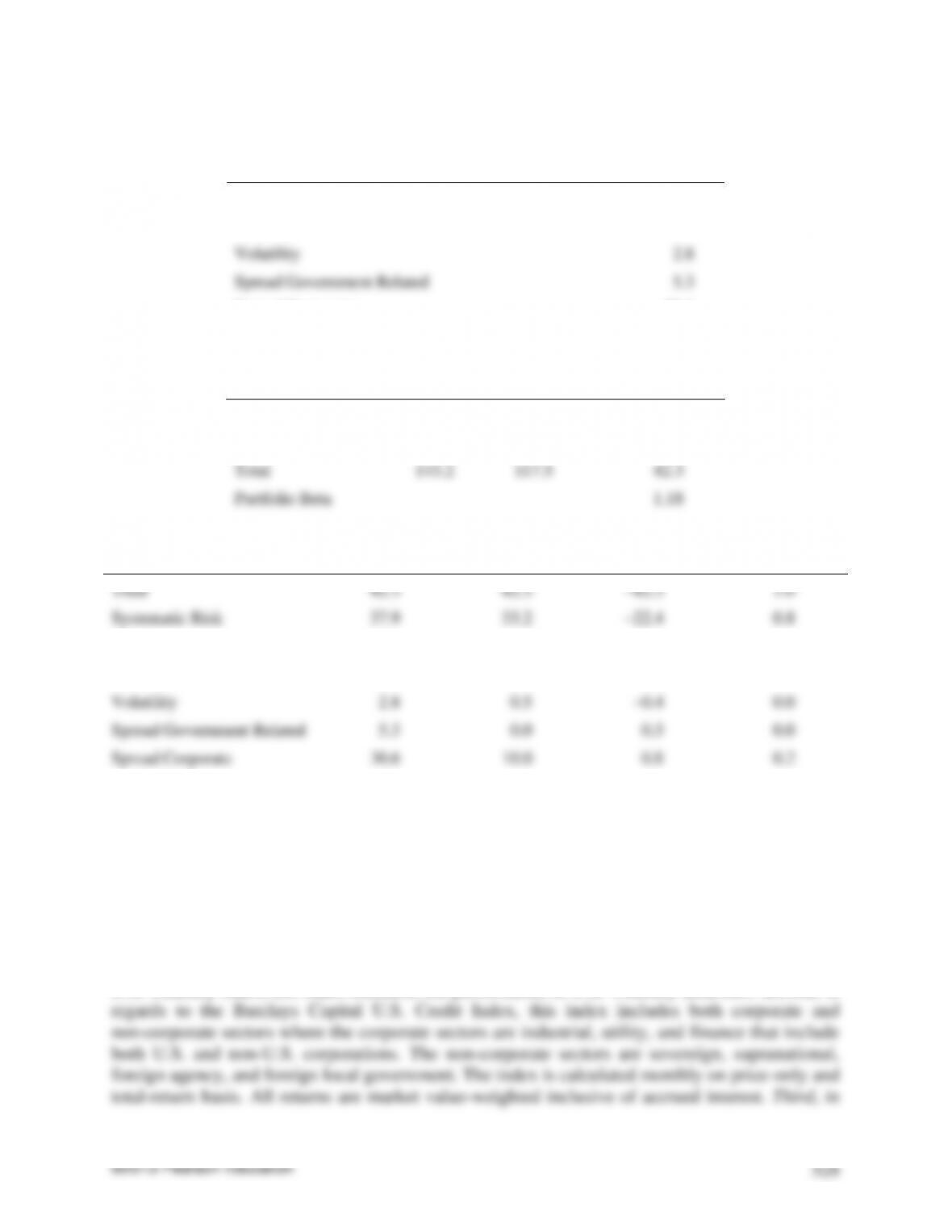
Risk Factor Categories
Risk
Curve
40.8
Swap Spreads
2.5
Volatility
2.8
Spread Government Related
5.3
Spread Corporate
30.6
Spread Securitized
5.8
Volatility
Portfolio
Benchmark
Tracking Error
Systematic
141.9
117.4
37.9
Idiosyncratic
19.3
4.8
18.7
Total
143.2
117.5
42.3
Portfolio Beta
1.18
Risk Factor Group
Isolated TEV
Contribution to
TEV
Liquidation
Effect on TEV
TEV Elasticity
(%)
Total
42.3
42.3
–42.3
1.0
Systematic Risk
37.9
33.2
–22.4
0.8
Curve
40.8
23.4
–4.3
0.5
Swap Spreads
2.5
0.2
–0.1
0.0
Volatility
2.8
0.5
–0.4
0.0
Spread Government Related
5.3
0.0
0.3
0.0
Spread Corporate
30.6
10.0
0.8
0.2
Spread Securitized
5.8
–0.8
1.1
0.0
Idiosyncratic Risk
18.7
9.1
–4.2
0.2
Describe in detail the risk characteristics of this portfolio. Be sure to discuss where it seems
like the manager is taking views on the market?
The benchmark for the manager who has constructed this portfolio is a composite index
consisting of one-third each of the Barclays Capital U.S. Treasury index, Barclays Capital U.S.
Credit Index, and Barclays Capital U.S. MBS index. First, in regards to the Barclays Capital
U.S. Treasury index, this index measures the performance of U.S. Treasury securities. Second, in
regards to the Barclays Capital U.S. MBS index, this index measures the performance of
investment grade fixed-rate mortgage-backed pass-through securities of GNMA, FNMA, and
FHLMC.
The analysis of the portfolio begins with a comparison of the portfolio to that of the benchmark.
Identification of the mismatches indicates where the manager has taken a view (unintentional or
not). The “asset class” table compares the portfolio and the benchmark in terms of the allocation
Although the information contained in the “asset” table (about the allocation based on percentage
market value of sector relative to the benchmark) provides a good starting point for our analysis,
the information has limited value because it is not known how the exposures to the sectors are
related to the exposures to the risk factors that drive the portfolio’s return. Here are three
examples. First, consider the Treasury sector. It is possible that the specific Treasury securities
contained in the portfolio have a lesser contribution to portfolio duration than the contribution to
It is for this reason that the portfolio manager must look beyond a naïve assessment of portfolio
risk relative to the benchmark based on percentage allocation to sectors. The “analytics” table
provides information about the relative exposure to interest rate risk as measured by duration,
spread risk as measured by spread duration, and call/prepayment risk as measured by vega, as
well as the convexity. From these analytics we observe the following:

The analysis thus far is missing a vital element. To understand why, suppose that a portfolio has
more exposure to a risk factor than the benchmark. This would mean if that risk factor moves,
the portfolio will have a greater movement than the benchmark. But the question is: To what
extent does that risk factor move? Another way of asking this is: How volatile is the risk factor?
For example, from the analysis of the analytics, we know that the portfolio has greater exposure
than the benchmark to changes in the level of interest rates (i.e., a higher duration) but less
exposure to changes in spreads (i.e., a higher spread duration). But which exposure (i.e., risk
factor) has greater volatility?
143.2 and 117.5, respectively.
Notice that for the benchmark, the percentage of the total risk (117.5) that is explained by the
18.7 basis points per month, respectively. The portfolio tracking error is
Portfolio tracking error = [(Systematic TE)2 + (Idiosyncratic TE)2]0.5
Therefore, the portfolio tracking error is 42.3 basis points per month. Consequently, although
©2013 Pearson Education
531
to a benchmark, there is tracking error risk of 42.3 basis points per month. (The systematic risk is
responsible for 18.7/42.3 or 44.21% of the total risk.)
This is an extremely important point: It is the tracking error not the idiosyncratic risk (as
measured by the standard deviation of the idiosyncratic returns) that the manager must consider
in portfolio construction and monitoring. In our illustration, the portfolio tracking error is small,
only 42.3 basis points.
As with equities where a portfolio beta is computed that shows the movement of an equity
portfolio in response to a movement in some equity market index (such as the S&P 500), a beta
can be computed for a bond portfolio. As shown in “volatility” table, the portfolio beta is 1.18.
(1) categories of risk factors and (2) asset classes (i.e., sectors of the benchmark).
This “risk factor group” table provides information about the portfolio risk across the different
categories of risk factors. Shown are the systematic risk and the idiosyncratic risk and six
components of systematic risk. The “contribution to TEV” column shows the isolated tracking