Chapter 23 – Futures, Swaps, and Risk Management
23-1
CHAPTER 23: FUTURES, SWAPS, AND RISK MANAGEMENT
PROBLEM SETS
1. In formulating a hedge position, a stock’s beta and a bond’s duration are used similarly to
determine the expected percentage gain or loss in the value of the underlying asset for a
given change in market conditions. Then, in each of these markets, the expected percentage
change in value is used to calculate the expected dollar change in value of the stock or
bond portfolios, respectively. Finally, the dollar change in value of the underlying asset,
along with the dollar change in the value of the futures contract, determines the hedge
ratio.
The major difference in the calculations necessary to formulate a hedge position in each
market lies in the manner in which the first step identified above is computed. For a hedge
in the equity market, the product of the equity portfolio’s beta with respect to the given
A secondary difference in the calculations necessary to formulate a hedge position in
each market arises in the calculation of the hedge ratio. In the equity market, the hedge
ratio is typically calculated by dividing the total expected dollar change in the value of
Chapter 23 – Futures, Swaps, and Risk Management
2. One of the considerations that would enter into the hedging strategy for a U.S. exporting
firm with outstanding bills to its customers denominated in foreign currency is whether
the U.S. firm also has outstanding payables denominated in the same foreign currency.
Since the firm receives foreign currency when its customers’ bills are paid, the firm
hedges by taking a short position in the foreign currency. The U.S. firm would reduce its
short position in futures to the extent that outstanding payables offset outstanding
receivables with the same maturity because the outstanding payables effectively hedge
3. The hedge will be much more effective for the gold-producing firm. Prices for distant
maturity oil futures contracts have surprisingly low correlation with current prices because
convenience yields and storage costs for oil can change dramatically over time. When
near-term oil prices fall, there may be little or no change in longer-term prices, since oil
23-3
4. Municipal bond yields, which are below T-bond yields because of their tax-exempt
status, are expected to close in on Treasury yields. Because yields and prices are
5. a. S0 (1 + rM ) − D = (1,425 1.06) – 15 = 1,495.50
c. The futures price is too low. Buy futures, short the index, and invest the proceeds
of the short sale in T-bills:
CF Now
CF in 6 months
Buy futures
0
S T − 1,422
Short index
1,425
−S T − 15
Buy T-bills
−1,425
1,467.75
Total
0
30.75
6. a. The value of the underlying stock is:
$250 1,350 = $337,500
c. $0.15/$0.0030 = 50
Chapter 23 – Futures, Swaps, and Risk Management
23-4
7. a. You should be short the index futures contracts. If the stock value falls, you need
b. Each contract is for $250 times the index, currently valued at 1,350. Therefore,
each contract controls stock worth: $250 1,350 = $337,500
c. Now, your stock swings only 0.6 as much as the market index. Hence, you need
8. If the beta of the portfolio were 1.0, she would sell $1 million of the index. Because beta
9. You would short $0.50 of the market index contract and $0.75 of the computer industry
10. The dollar is depreciating relative to the euro. To induce investors to invest in the U.S.,
06.1
04.1
r1
r1
UK
US
00 ==
+
+
b. Suppose that F0 = $2.03/£. Then dollars are relatively too cheap in the forward
market, or equivalently, pounds are too expensive. Therefore, you should borrow
the present value of £1, use the proceeds to buy pound-denominated bills in the
spot market, and sell £1 forward:
Action Now
CF in $
Action at period-end
CF in $
Sell £1 forward for $2.03
0
Collect $2.03,
deliver £1
$2.03 – $E1
Buy £1/1.06 in spot market;
invest at the British risk-free rate
–2.00/1.06 = –$1.887
Exchange £1 for $E1
$E1
Borrow $1.887
$1.887
Repay loan;
U.S. interest rate = 4%
–$1.962
Total
0
Total
$0.068
Chapter 23 – Futures, Swaps, and Risk Management
23-5
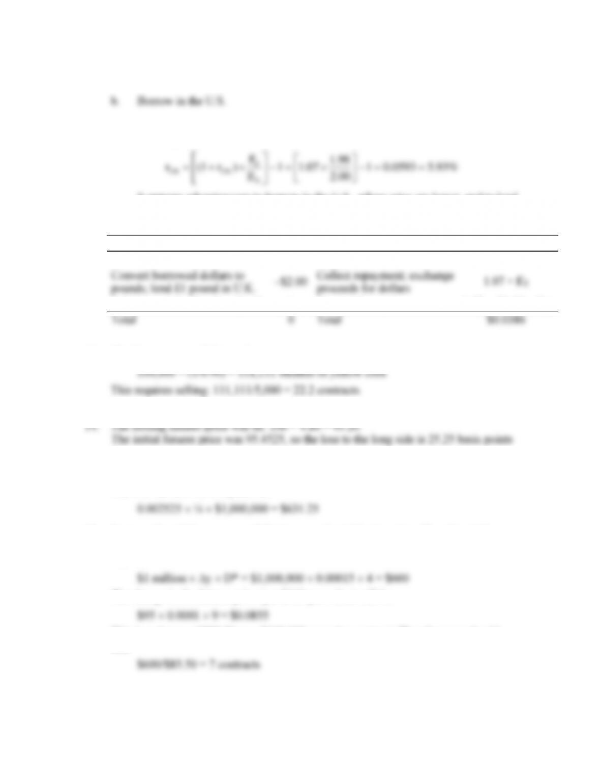
12. a. Lend in the U.K.
c. Borrowing in the U.S. offers a 4% rate of return. Borrowing in the U.K. and
covering interest rate risk with futures or forwards offers a rate of return of:
%93.50593.01
00.2
98.1
07.11
E
F
)r(1r
0
0
UKUS ==−
=−
+=
It appears advantageous to borrow in the U.S., where rates are lower, and to lend
in the U.K. An arbitrage strategy involves simultaneous lending and borrowing
with the covering of interest rate risk:
Action Now
CF in $
Action at period-end
CF in $
Borrow $2.00 in U.S.
$2.00
Repay loan
–$2.00 × 1.04
Convert borrowed dollars to
pounds; lend £1 pound in U.K.
–$2.00
Collect repayment; exchange
proceeds for dollars
1.07 × E1
Sell forward £1.07 at F0 = $1.98
0
Unwind forward
1.07 × ($1.98 – E1)
Total
0
Total
$0.0386
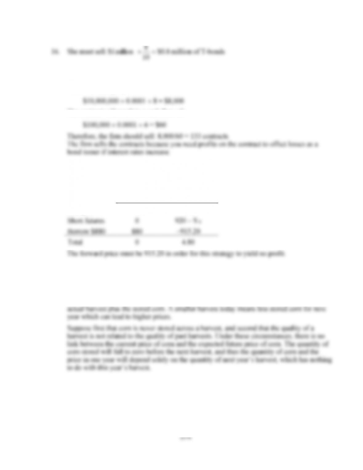
13. The farmer must sell forward:
or:
25.25 basis points $25 per basis point = $631.25
The loss can also be computed as:
15. Suppose the yield on your portfolio increases by 1.5 basis points. Then the yield on
the T-bond contract is likely to increase by 1 basis point. The loss on your portfolio
will be:
The change in the futures price (per $100 par value) will be:
This is a change of $85.50 on a $100,000 par value contract. Therefore you should
sell:
Chapter 23 – Futures, Swaps, and Risk Management
23-6
16. She must sell:
8.0$
10
8
million 1$ =
million of T-bonds
17. If yield changes on the bond and the contracts are each 1 basis point, then the bond
value will change by:
The contract will result in a cash flow of:
18. F0 = S0(l + rf )T = 880 1.04 = 915.20
If F0 = 920, you could earn arbitrage profits as follows:
CF Now
CF in 1 year
Buy gold
−880
S T
Short futures
0
920 − S T
Borrow $880
880
−915.20
Total
0
4.80
The forward price must be 915.20 in order for this strategy to yield no profit.
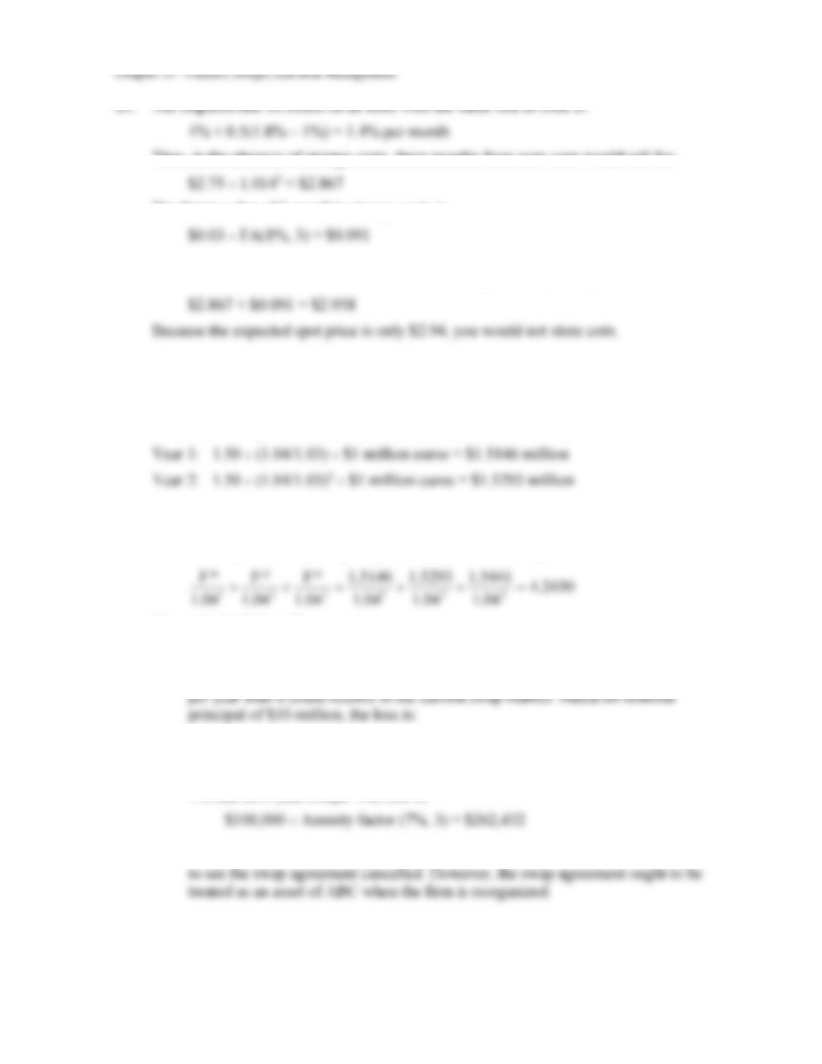
19. If a poor harvest today indicates a worse than average harvest in future years, then the futures
prices will rise in response to today’s harvest, although presumably the two-year price will
change by less than the one-year price. The same reasoning holds if corn is stored across the
harvest. Next year’s price is determined by the available supply at harvest time, which is the
23-7
Thus, in the absence of storage costs, three months from now corn would sell for:
The future value of 3 month’s storage costs is:
where FA stands for the future value factor for a level annuity with a given interest rate and
number of payments. Thus, in order to induce storage, the expected price would have to be:
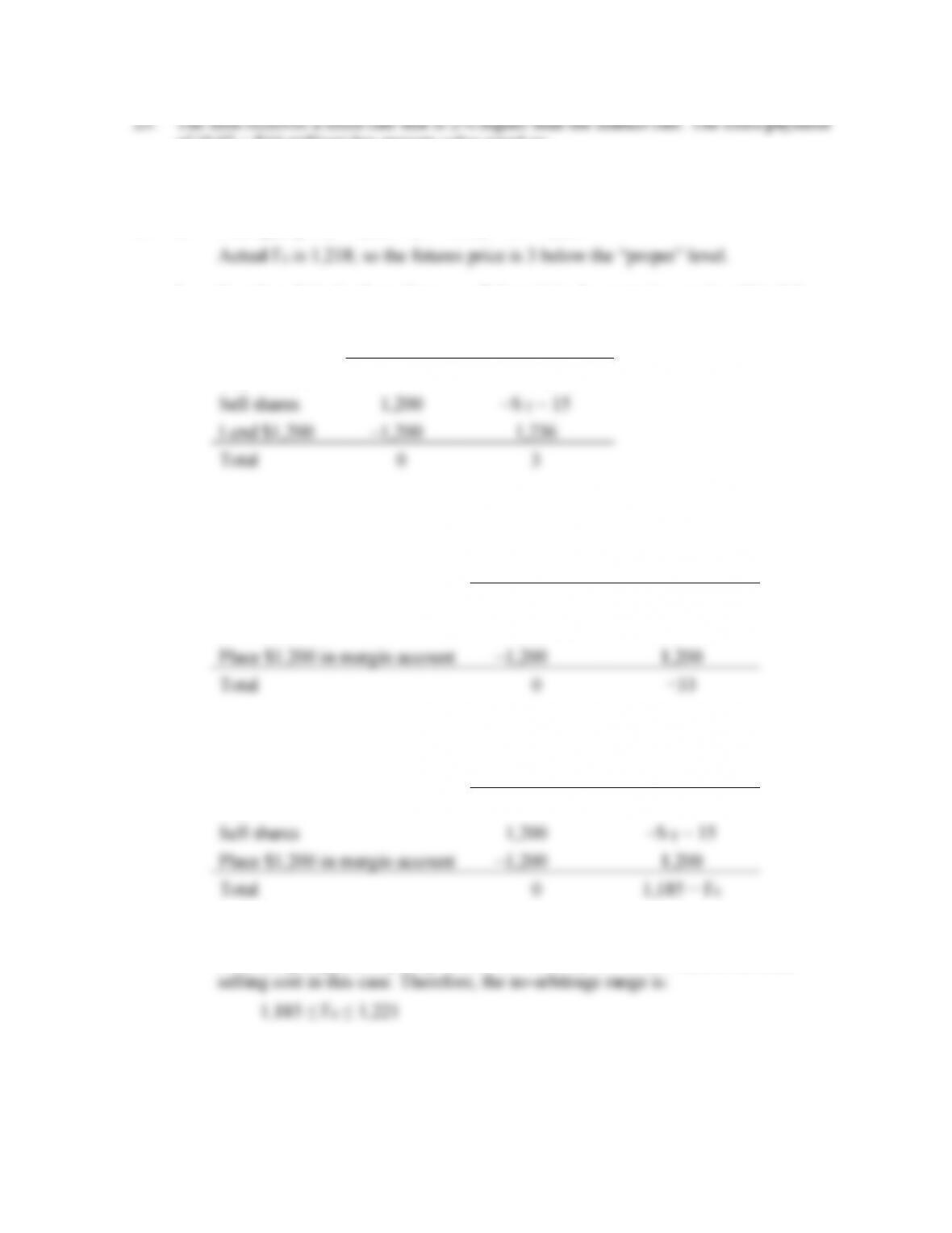
21. If the exchange of currencies were structured as three separate forward contracts, the
forward prices would be determined as follows:
Forward exchange rate $1 million euros = dollars to be delivered
Year 3: 1.50 (1.04/1.03)3 $1 million euros = $1.5441 million
Instead, we deliver the same number of dollars (F*) each year. The value of F* is
determined by first computing the present value of this obligation:
2430.4
04.1
5441.1
04.1
5293.1
04.1
5146.1
1.04
*F
1.04
*F
1.04
*F
321321 =++=++
F* equals $1.5290 million per year.
22. a. The swap rate moved in favor of firm ABC. ABC should have received 1% more
0.01 $10 million = $100,000 per year.
b. The market value of the fixed annual loss is obtained by discounting at the current
7% rate on 3-year swaps. The loss is:
c. If ABC had become insolvent, XYZ would not be harmed. XYZ would be happy
Chapter 23 – Futures, Swaps, and Risk Management
23-8
of (0.02 × $10 million) has present value equal to:
$200,000 × Annuity factor (8%, 5) = $799,542
24. a. From parity: F0 = 1,200 (1 + 0.03) – 15 = 1,221
b. Buy the relatively cheap futures, sell the relatively expensive stock and lend the
proceeds of the short sale:
CF Now
CF in 6 months
Buy futures
0
S T − 1,218
Sell shares
1,200
−S T − 15
Lend $1,200
−1,200
1,236
Total
0
3
c. If you do not receive interest on the proceeds of the short sales, then the $1200 you
receive will not be invested but will simply be returned to you. The proceeds from
the strategy in part (b) are now negative: an arbitrage opportunity no longer exists.
CF Now
CF in 6 months
Buy futures
0
S T − 1,218
Sell shares
1,200
−S T − 15
Place $1,200 in margin account
−1,200
1,200
Total
0
−33
d. If we call the original futures price F0 , then the proceeds from the long-futures,
short-stock strategy are:
CF Now
CF in 6 months
Buy futures
0
S T − F0
Sell shares
1,200
−S T − 15
Place $1,200 in margin account
−1,200
1,200
Total
0
1,185 − F0
Therefore, F0 can be as low as 1,185 without giving rise to an arbitrage
opportunity. On the other hand, if F0 is higher than the parity value (1,221), then
an arbitrage opportunity (buy stocks, sell futures) will exist. There is no short-
Chapter 23 – Futures, Swaps, and Risk Management
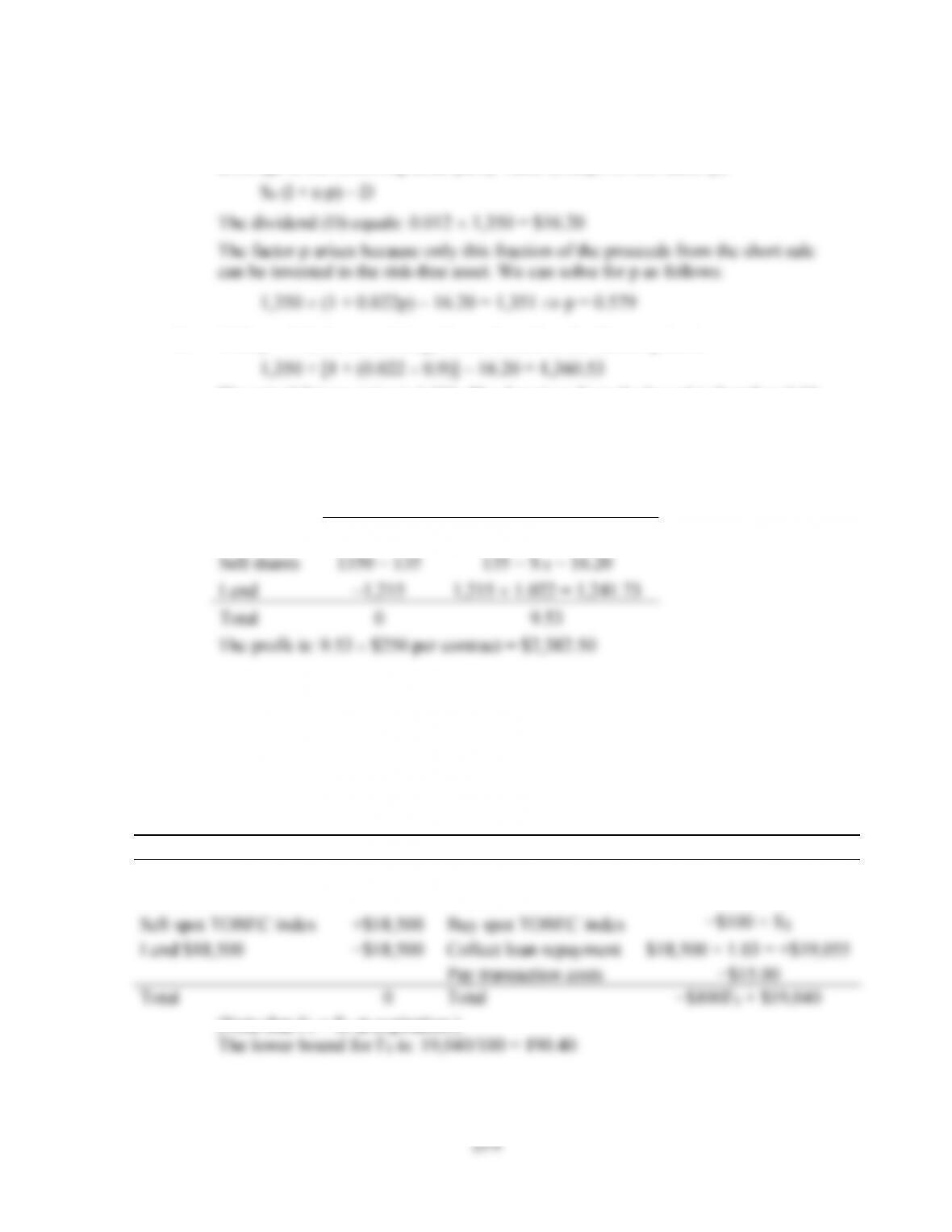
25. a. Call p the fraction of proceeds from the short sale to which we have access.
Ignoring transaction costs, the lower bound on the futures price that precludes
arbitrage is the following usual parity value (except for the factor p):
b. With p = 0.9, the no-arbitrage lower bound on the futures price is:
The actual futures price is 1,351. The departure from the bound is therefore 9.53.
This departure also equals the potential profit from an arbitrage strategy. The strategy
is to short the stock, which currently sells at 1,350. The investor receives 90% of the
proceeds (1,215) and the remainder (135) remains in the margin account until the
short position is covered in 6 months. The investor buys futures and lends 1,215:
CF Now
CF in 6 months
Buy futures
0
S T − 1,351
Sell shares
1350 − 135
135 − S T − 16.20
Lend
−1,215
1,215 1.022 = 1,241.73
Total
0
9.53
The profit is: 9.53 $250 per contract = $2,382.50
CFA PROBLEMS
1. a. By spot-futures parity:
F0 = S0 × (l + rf ) = 185 × [1 + (0.06/2)] = 190.55
b. The lower bound is based on the reverse cash-and-carry strategy.
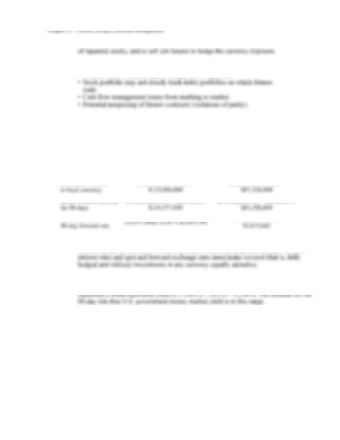
Action Now
CF in $
Action at period-end
CF in $
Buy one TOBEC index
futures contract
0
Sell one TOBEC index
futures contract
$100 × (F1 − F0)
Sell spot TOBEC index
+$18,500
Buy spot TOBEC index
−$100 × S1
Lend $18,500
−$18,500
Collect loan repayment
$18,500 × 1.03 = +$19,055
Pay transaction costs
−$15.00
Total
0
Total
−$100F0 + $19,040
(Note that F1 = S1 at expiration.)
23–10
2. a. The strategy would be to sell Japanese stock index futures to hedge the market risk
b. Some possible practical difficulties with this strategy include:
• Contract size on futures may not match size of portfolio.
3. a. The hedged investment involves converting the $1 million to foreign currency,
investing in that country, and selling forward the foreign currency in order to lock
in the dollar value of the investment. Because the interest rates are for 90-day
periods, we assume they are quoted as bond equivalent yields, annualized using
simple interest. Therefore, to express rates on a per quarter basis, we divide these
rates by 4:
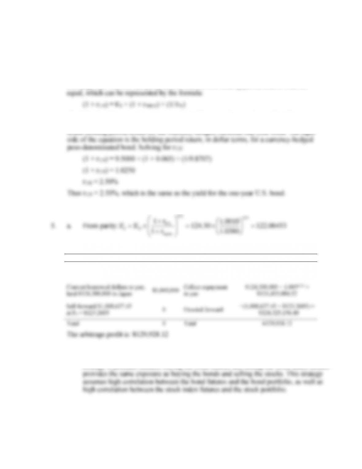
Japanese government
Swiss government
Convert $1 million
to local currency
$1,000,000 × 133.05 =
¥133,050,000
$1,000,000 × 1.5260 =
SF1,526,000
Invest in local currency
for 90 days
¥133,050,000 × [1 + (0.076/4)] =
¥135,577,950
SF1,526,000 × [1 + (0.086/4)] =
SF1,558,809
Convert to $ at
90-day forward rate
135,577,950/133.47 = $1,015,793
1,558,809/1.5348 =
$1,015,643
b. The results in the two currencies are nearly identical. This near-equality reflects the
interest rate parity theorem. This theory asserts that the pricing relationships between
c. The 90-day return in Japan is 1.5793%, which represents a bond-equivalent yield of
1.5793% 365/90 = 6.405%. The 90-day return in Switzerland is 1.5643%, which
Chapter 23 – Futures, Swaps, and Risk Management
23–11
4. The investor can buy X amount of pesos at the (indirect) spot exchange rate, and invest the
pesos in the Mexican bond market. Then, in one year, the investor will have:
X × (1 + r MEX) pesos
These pesos can then be converted back into dollars using the (indirect) forward
exchange rate. Interest rate parity asserts that the two holding period returns must be
The left side of the equation represents the holding period return for a U.S. dollar-
denominated bond. If interest rate parity holds, then this term also corresponds to the U.S.
dollar holding period return for the currency-hedged Mexican one-year bond. The right
0380.1
0010.1
r1
r1
5.0
5.0
Japan
US
00 =
+
+
b.
Action Now
CF in $
Action at period-end
CF in ¥
Borrow $1,000,000 in U.S.
$1,000,000
Repay loan
−($1,000,000 × 1.0350.25 ) =
−$1,008,637.45
Convert borrowed dollars to yen;
lend ¥124,300,000 in Japan
–$1,000,000
Collect repayment
in yen
¥124,300,000 × 1.0050.25 =
¥124,455,084.52
Sell forward $1,008,637.45
at F0 = ¥123.2605
0
Unwind forward
−(1,008,637.45 × ¥123.2605) =
−¥124,325,156.40
Total
0
Total
¥129,928.12
The arbitrage profit is: ¥129,928.12
6. a. Delsing should sell stock index futures contracts and buy bond futures contracts. This
strategy is justified because buying the bond futures and selling the stock index futures
Chapter 23 – Futures, Swaps, and Risk Management
23–12
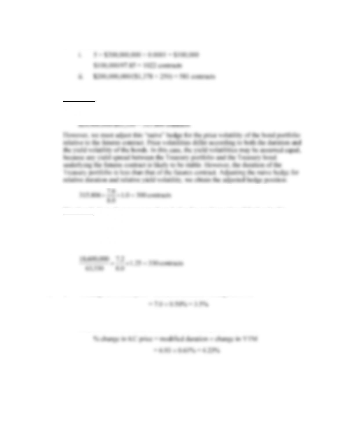
b. The number of contracts in each case is:
7. Situation A. The market value of the portfolio to be hedged is $20 million. The market
value of the bonds controlled by one futures contract is $63,330. If we were to equate the
market values of the portfolio and the futures contract, we would sell:
0.8
Situation B. Here, the treasurer seeks to hedge the purchase price of the bonds; this
requires a long hedge. The market value of the bonds to be purchased is:
$20 million 0.93 = $18.6 million
The duration ratio is 7.2/8.0, and the relative yield volatility is 1.25. Therefore, the hedge
requires the treasurer to take a long position in:
33025.1
0.8
2.7
330,63
000,600,18 =
contracts
8. a. % change in T-bond price = modified duration change in YTM
b. When the YTM of the T-bond changes by 50 basis points, the predicted change in
the yield on the KC bond is 1.22 50 = 61 basis points. Therefore: