
CHAPTER 23
BOND PORTFOLIO CONSTRUCTION
CHAPTER SUMMARY
In this chapter, we will see how to construct (build) portfolios. We begin with a brief review of
the basic principles of the theory of portfolio selection and portfolio risk. Then we explain a key
metric used in constructing, monitoring, and controlling portfolio risk: tracking error. In the last
two sections of the chapter we then explain two approaches to portfolio construction: cell-based
approach and multi-factor model approach.
BRIEF REVIEW OF PORTFOLIO THEORY AND RISK DECOMPOSITION
Portfolio theory as formulated by Harry Markowitz in the early 1950s provides guidance for the
construction of portfolios. The Markowitz framework, also referred to as mean-variance
analysis, states there are three parameters that are important in making portfolio selection
where
E(R1 ), E(R2), and E(Rp) are the expected return of asset 1, asset 2, and the portfolio, respectively.
w1and w2 are the weight (allocation) of assets 1 and 2, respectively, in the portfolio at the
beginning of the period
( ) ( )
12
SD / SD
©2013 Pearson Education
503
where cor(R1, R2) is the correlation between the return of asset 1 and asset 2, and SD(R1) and
SD(R2) are the standard deviation of the return of asset 1 and asset 2, respectively. Rearranging
the above equation, we have:
Using this latter variance equation, it is easier to appreciate how the relationship between asset
returns as measured by the correlation impacts the portfolio variance. A correlation of zero
implies that the returns are uncorrelated. Let’s look at the following three cases:
The maximum portfolio variance occurs when there is perfect correlation (i.e., correlation of +1)
between the return of the two assets. The minimum portfolio variance occurs when asset returns
have a correlation of –1.
APPLICATION OF PORTFOLIO THEORY TO BOND PORTFOLIO CONSTRUCTION
The Markowitz mean-variance framework has been applied to portfolio construction in two
ways. The first is at the asset class level. The second application is the use of the mean-variance
framework to select securities to construct portfolio.
©2013 Pearson Education
504
The use of portfolio variance as a risk measure is an issue for two reasons. The first is that it is
assumed that the return distribution for securities is normally distributed. If this holds, the
variance is the appropriate measure of risk. However, empirical and theoretical evidence
suggests that stock returns and bond returns are not normally distribution. The second attack on
portfolio variance is one that follows from a discussion about the objective of portfolio
managers: outperforming a benchmark. The measure used with this objective is a portfolio’s
tracking error. This measure is the standard deviation or variance of the difference between the
portfolio return and the benchmark return. The key point is that in constructing a portfolio where
there is a benchmark, the relevant risk measure is not the portfolio variance but the portfolio
tracking error.
TRACKING ERROR
When a portfolio manager’s benchmark is a bond market index, risk is not measured in terms of
the variance or standard deviation of the portfolio’s return. Instead, risk is measured by the
standard deviation of the return of the portfolio relative to the return of the benchmark index.
This risk measure is called tracking error. Tracking error is also called active risk.
at79.13 basis points.
A tracking error is annualized when observations are monthly as follows:
annual tracking error 5 monthly tracking error ×
12
Two Faces of Tracking Error
We call tracking error calculated from observed active returns for a portfolio backward-looking
tracking error. It is also called ex-post tracking error, historical tracking error, and actual
tracking error.A problem with using backward-looking tracking error in bond portfolio
management is that it does not reflect the effect of current decisions by the portfolio manager on
the future active returns and hence the future tracking error that may be realized.
Given a forward-looking tracking error, a range for the future possible portfolio active return can
be calculated assuming that the active returns are normally distributed. For example, assume the
following:
Tracking Error and Active versus Passive Strategies
A passive strategy relative to the benchmark index occurs when a forward-looking tracking error
is very small. When the forward-looking tracking error is large, the manager is pursuing an
active strategy.
CELL-BASED APPROACH TO BOND PORTFOLIO CONSTRUCTION
Under the cell-based approach to constructing a bond portfolio, the benchmark is divided into
cells, each cell representing a different characteristic of the benchmark. The most common cells

For a portfolio manager pursuing a passive strategy, the objective is to match the performance of
the benchmark. Following the cell-based approach, the manager selects from all the issues in the
bond index one or more issues in each cell that can be used to represent the entire cell. The total
Complications in Bond Indexing
There are three forms of bond indexing: pure bond index matching, enhanced indexing matching
primary risk factors, and enhanced indexing allowing for minor risk-factor mismatches. It almost
impossible to implement a pure bond indexing strategy and it is not simple to do so for the other
There are logistical problems unique to certain sectors in the bond market. Because of the
illiquidity of this sector of the bond market, not only may the prices used by the organization that
publishes the index be unreliable, but many of the issues may not even be available. Next,
consider the agency mortgage-backed securities market. There are more than 800,000 agency
PORTFOLIO CONSTRUCTION WITH MULTI-FACTOR MODELS
Multi-factor models are statistical models that are used to estimate a security’s expected return
based on the primary drivers affecting the return on securities. The primary drivers of returns are
Risk Decomposition
Exhibit 23-3 illustrates how a multi-factor model can be used to identify the risk exposure of
a portfolio relative to a benchmark. This portfolio was constructed using a multi-factor model
combined with an optimization model. The risk exposure for this portfolio is measured in terms
of tracking error. The analysis of the portfolio begins with a comparison of the portfolio to that
of the benchmark.
Although the information contained in Exhibit 23-4 about the allocation based on percentage
market value of sector relative to the benchmark provides a good starting point for our analysis,
the information has limited value because it is not known how the exposures to the sectors are
More information about the portfolio’s relative risk exposure to interest rate risk can be obtained
by looking at the contribution to duration for the portfolio and the benchmark. This is shown in
Exhibit 23-6. As can be seen, the major reason for the slightly longer duration of the portfolio
relative to the benchmark is mainly attributable to the duration of the Treasury securities selected
for the portfolio.

squaring each isolated tracking error for each risk factor, summing them, and then taking the
square root. That is, for the general case where there are K risk factors is
Portfolio isolated systematic TE = [(TE1)2 + (TE2)2 + … + (TEK)2]1/2
The portfolio tracking error is
Portfolio tracking error = [(Systematic TE)2 + (Idiosyncratic TE)2]0.5
An extremely important point is that the tracking error (and not the idiosyncratic risk) is what the
manager must consider in portfolio construction and monitoring.
As with equities where a portfolio beta is computed that shows the movement of anequity
portfolio in response to a movement in some equity market index (such as the S&P500), a beta
can be computed for a bond portfolio.A beta-type measure can be estimated for each risk factor.
For example, consider the risk factor measuring changes in the level of the yield curve which is
the portfolio’s duration. A duration beta can be calculated as follows:
Portfolio duration
Duration beta Benchmark duration
=
A detailed analysis of the systematic and idiosyncratic risk applied at the asset class level rather
than at the individual risk factor level is provided in Exhibit 23-10. The five asset classes are
shown in the first column and in the second column the underweighting or overweighting of each
An analysis similar to the decomposition of risk shown in Exhibit 23-9 by asset class instead of
risk factor group is shown in Exhibit 23-11. Notice that the isolated tracking error for both the
Treasury and corporate asset classes exceeds that of the portfolio tracking error. This occurs
In the Barclays Capital model, there is a different yield curve used for government products.
With the exception of Treasuries, the other asset classes have exposure to the swap spread factors
on top of the Treasury curve. By decomposing the swap curve into the Treasury curve and swap
spreads, the Barclays Capital model gives portfolio managers the flexibility to analyze their
spread risk over the Treasury or the swap curve depending on their preferences.
Exhibit 23-13 shows the exposure of the portfolio to the change in the swap spread. The swap
spread is the difference between the swap rate and the Treasury rate. All securities in the
portfolio except Treasuries expose the portfolio to this risk.
Portfolio Construction Using a Multi-Factor Model and an Optimizer
As with the cell-based approach to portfolio construction, a manager has views on the various
primary factors driving the return on the benchmark and wants to position the portfolio to
capitalize on those expectations.A multi-factor model is used in conjunction with an optimizer to

Portfolio Rebalancing
While it is common to illustrate portfolio construction starting with a position of cash and
building a portfolio of securities, in practice the more common task is to rebalance an existing
portfolio. A multi-factor model along with an optimizer can be used to efficiently rebalance the
KEY POINTS
• The Markowitz mean-variance model is used to construct portfolios. The inputs required are
the mean (expected return) and variance for each security that is a candidate for inclusion in
the portfolio and the covariance or correlation between each pair of securities.
• While the insights provided by Markowitz mean-variance model are important, there are
several issues that limit its application to the construction of bond portfolios.
• Tracking error, or active risk, is the standard deviation of a portfolio’s return relative to the
benchmark index.

©2013 Pearson Education
511
• The systematic risk factors in multi-factor model include yield curve risk, swap spread risk,
volatility risk, government-related spread risk, corporate spread risk, and securitized spread
risk.
• The risk exposure in a factor model is measured in terms of tracking error.
• Multi-factor models combined with an optimization model are used to construct a portfolio
that minimizes tracking error subject to the constraints imposed by the manager (client
imposed or self imposed) and embodying the views of the manager.
ANSWERS TO QUESTIONS FOR CHAPTER 23
(Questions are in bold print followed by answers.)
1. What is the major insight provided by the Markowitz framework in portfolio theory?
The main insight of the Markowitz framework is that when assets are combined to create
a portfolio, the portfolio’s risk (as measured by the portfolio variance) is not merely some
weighted average of the risks of the individual assets comprising the portfolio. Instead, the
2. Answer the below questions.
a. Explain whether you agree or disagree with the following statement: “It is the covariance
not the correlation that is important in the mean-variance model for portfolio selection.”
One would disagree with the statement because the covariance and correlation can be defined in
terms of one another. Specifically, the correlation between the returns for two assets is equal to
b. Explain whether you agree or disagree with the following statement: “In the
mean-variance framework, the variance is lower the higher the correlation between the assets in
the portfolio.”
Consider the below equation representing a simple portfolio of two assets (asset 1 and asset 2):
3. What are the two ways in which the Markowitz mean-variance framework has been used
by investors?
The Markowitz mean-variance framework has been applied to portfolio construction in two ways.
The first is at the asset class level where investors make an asset allocation decision. This is the
decision as to how to allocate funds amongst the major asset classes (stocks, bonds, cash, real
estate, and alternative assets). This has probably been the major use of the Markowitz framework.
4. What are the difficulties of implementing the Markowitz mean-variance framework in
constructing portfolios?
The implementation for constructing portfolios requires the estimation of the inputs (mean,
variance, and covariance) for all of the securities that are candidates for inclusion in the
portfolio. These inputs are not easily estimated and this presents a variety of difficulties. For
example, the number of inputs that must be calculated is enormous. For example, if there are
N securities that can be included in a portfolio, there are N variances and (N2– N)/2 covariances
to estimate. Hence, for a portfolio of just 50 securities that could be included in a portfolio, there
are 1,224 covariances that must be calculated. For 100 securities, there are 4,950 covariances.
©2013 Pearson Education
514
take more than 25 or so randomly selected stocks to remove most of the idiosyncratic risk of a
portfolio. That is, a randomly selected portfolio of stocks is mostly exposed to systematic risk.
However, when risk is measured in terms of tracking error, it takes a considerably larger number
of stocks to remove idiosyncratic risk. Typically, this is not the case when dealing with bonds
where the benchmark is one of the standard bond market indexes.
5. What was the purpose for William Sharpe’s development of the single index market model?
It was clear to Markowitz that some kind of model of covariance structure was needed for the
practical implementation of the theory to large portfolios. He did little more than point out the
problem and suggest some possible models of covariance. One model Markowitz proposed to
explain the correlation structure among security returns assumed that the return on a security
6. Why is the tracking error more important than portfolio variance of returns when a
portfolio manager’s performance is measured versus a benchmark?
A key point is that in constructing a portfolio where there is a benchmark, the relevant risk
measure is not the portfolio variance but the portfolio tracking error. When performance is
measured against a benchmark, tracking error is more important than portfolio variance
because on tracking error measures how closely a portfolio follows the index to which it is
benchmarked. The most common measure is the root-mean-square of the difference between the
portfolio and index returns.
7. What is tracking error?
When a portfolio manager’s benchmark is a bond market index, risk is not measured in terms of
the standard deviation of the portfolio’s return. Instead, risk is measured by the standard
deviation of the return of the portfolio relative to the return of the benchmark index. This risk
©2013 Pearson Education
515
measure is called tracking error. Tracking error is also called active risk.
Tracking error is computed as follows. First, compute the total return for a portfolio for each
period. Second, obtain the total return for the benchmark index for each period. Third, obtain the
difference between the return values for portfolio and index for each period. The difference for
each period is referred to as the active return for that period. Finally, compute the standard
deviation of the active returns. The resulting value is the tracking error.
One should not that the tracking error measurement is in terms of the observation period. If
monthly returns are used, the tracking error is a monthly tracking error. If weekly returns are
used, the tracking error is a weekly tracking error. Tracking error is annualized as follows. When
observations are monthly: annual tracking error= monthly tracking error ×
12
. When
observations are weekly: annual tracking error = monthly tracking error ×
52
.
8. Explain why backward-looking tracking error has limitations for estimating a portfolio’s
future tracking error.
A portfolio’s backward-looking tracking error is computed based on actual active returns and
9. Why might one expect that for a manager pursuing an active management strategy that
the backward-looking tracking error at the beginning of the year will deviate from the
forward-looking tracking error at the beginning of the year?
The portfolio manager needs a forward-looking estimate of tracking error to reflect the portfolio
risk going forward. The way this is done in practice is by using the services of a commercial
vendor or dealer firm that has modeled the factors that affect the tracking error associated with
10. Answer the below questions.
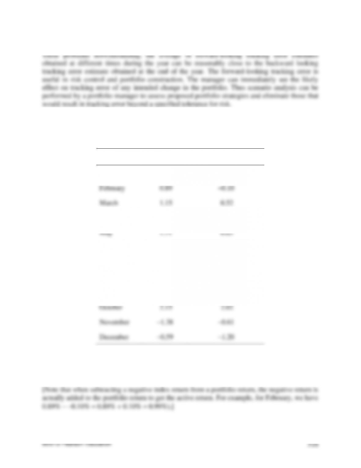
(a) Compute the tracking error from the following information:
Month 2001
Portfolio A’s
Return (%)
Lehman Aggregate
Bond Index Return (%)
January
2.15
1.65
February
0.89
–0.10
March
1.15
0.52
April
–0.47
–0.60
May
1.71
0.65
June
0.10
0.33
July
1.04
2.31
August
2.70
1.10
September
0.66
1.23
October
2.15
2.02
November
–1.38
–0.61
December
–0.59
–1.20
The tracking error is the standard deviation of the active returns where an active return is the
portfolio A’s return minus the benchmark’s return for each month. The below table has each
active return in the “Active Return” column.