Chapter 21 – Option Valuation
21-1
CHAPTER 21: OPTION VALUATION
PROBLEM SETS
1. The value of a put option also increases with the volatility of the stock. We see this
from the put–call parity theorem as follows:
2. A $1 increase in a call option’s exercise price would lead to a decrease in the
4. Holding beta constant, the stock with a lot of firm-specific risk has higher total
volatility. The option on the stock with higher firm-specific risk is worth more.
6. a. Put A must be written on the stock with the lower price. Otherwise, given the
lower volatility of Stock A, Put A would sell for less than Put B.
b. Put B must be written on the stock with the lower price. This would explain its
Chapter 21 – Option Valuation
21-2
7.
Exercise
Price
Hedge
Ratio
0/30 = 0.000
90
8.
S
d1
N(d1)
45
-0.2768
0.3910
50
0.2500
0.5987
55
0.7266
0.7662
9. a. uS 0 = 130 Pu = 0
b.
Riskless
Portfolio
ST = 80
ST = 130
Buy 3 shares
240
390
Buy 5 puts
150
Total
390
390
Chapter 21 – Option Valuation
10. The hedge ratio for the call is:
00
20 0 2
130 80 5
ud
CC
HuS dS
−−
= = =
−−
11. d1 = 0.2192 N(d1) = 0.5868
12. P = $6.60
13. a. C falls to $5.1443
b. C falls to $3.8801
Chapter 21 – Option Valuation
21-4
14. According to the Black-Scholes model, the call option should be priced at:
15. A straddle is a call and a put. The Black-Scholes value would be:
16. A. A delta-neutral portfolio is perfectly hedged against small price changes in the
underlying asset. This is true both for price increases and decreases. That is, the
17. A. Delta is the change in the option price for a given instantaneous change in the stock
price. The change is equal to the slope of the option price diagram.
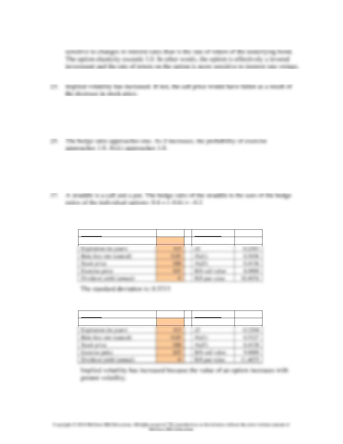
20. The number of calls needed to create a delta-neutral hedge is inversely proportional to
21. A delta-neutral portfolio can be created with any of the following combinations: long
Chapter 21 – Option Valuation
21-5
22. The rate of return of a call option on a long-term Treasury bond should be more
24. Implied volatility has increased. If not, the put price would have fallen as a result of
the decreased time to expiration.
26. The hedge ratio approaches 0. As X decreases, the probability of exercise
approaches 0. [N(d1) –1] approaches 0 as N(d1) approaches 1.
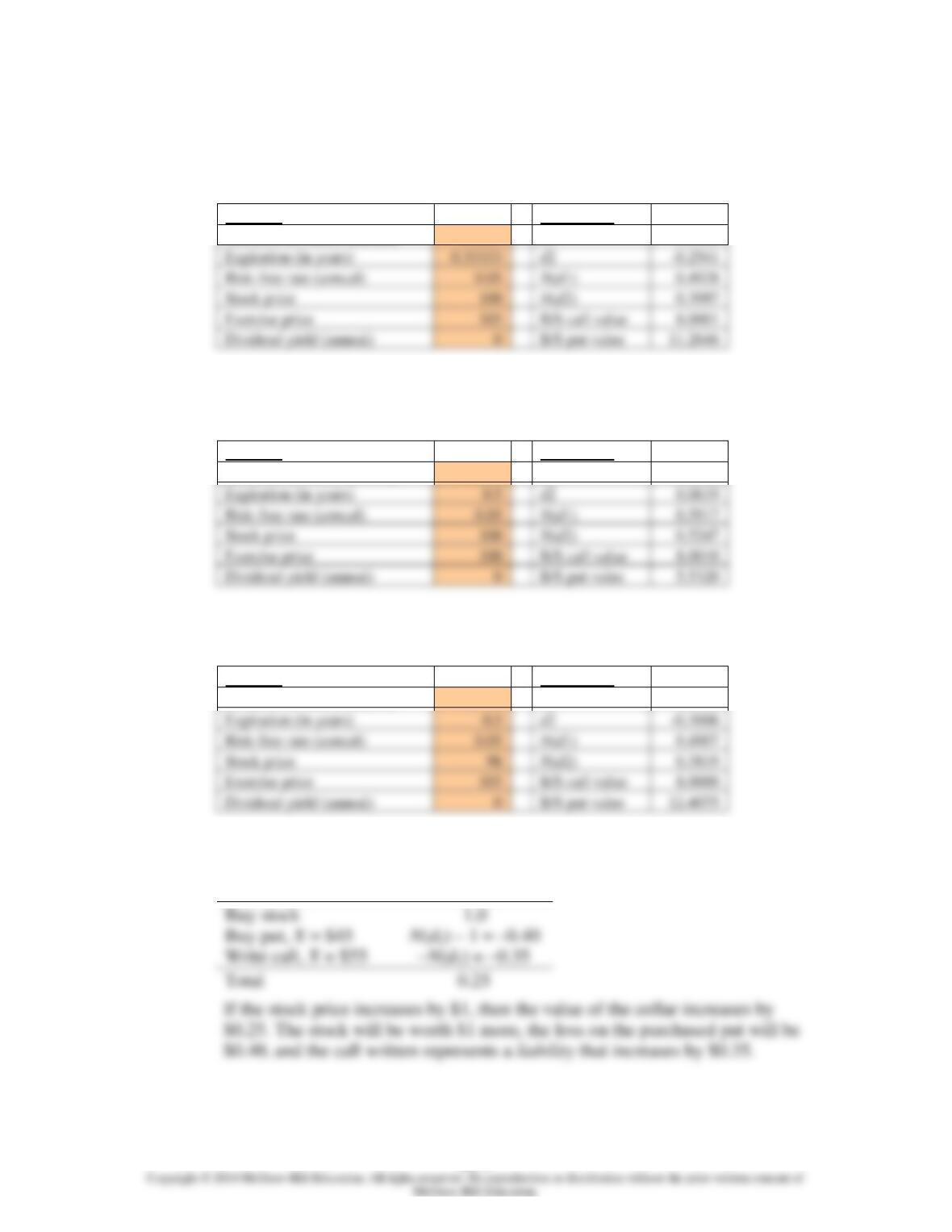
28. a. The spreadsheet appears as follows:
INPUTS
OUTPUTS
Standard deviation (annual)
0.3213
d1
0.0089
Expiration (in years)
d2
Risk-free rate (annual)
0.5036
Stock price
0.4136
Exercise price
B/S call value
8.0000
Dividend yield (annual)
B/S put value
INPUTS
OUTPUTS
Standard deviation (annual)
0.3568
d1
0.0318
Expiration (in years)
d2
Risk-free rate (annual)
0.5127
Stock price
0.4128
Exercise price
B/S call value
9.0000
Dividend yield (annual)
B/S put value
Chapter 21 – Option Valuation
21-6
c. Implied volatility increases to 0.4087 when expiration decreases to four
months. The shorter expiration decreases the value of the option; therefore, in
order for the option price to remain unchanged at $8, implied volatility must
increase.
INPUTS
OUTPUTS
Standard deviation (annual)
0.4087
d1
-0.0182
Expiration (in years)
Risk-free rate (annual)
Stock price
Exercise price
B/S call value
Dividend yield (annual)
B/S put value
d. Implied volatility decreases to 0.2406 when exercise price decreases to $100.
The decrease in exercise price increases the value of the call, so that, in order
for the option price to remain at $8, implied volatility decreases.
INPUTS
OUTPUTS
Standard deviation (annual)
0.2406
d1
0.2320
Expiration (in years)
Risk-free rate (annual)
Stock price
Exercise price
B/S call value
Dividend yield (annual)
B/S put value
5.5320
e. The decrease in stock price decreases the value of the call. In order for the
option price to remain at $8, implied volatility increases.
INPUTS
OUTPUTS
Standard deviation (annual)
0.3566
d1
-0.0484
Expiration (in years)
Risk-free rate (annual)
0.4807
Stock price
Exercise price
B/S call value
Dividend yield (annual)
B/S put value
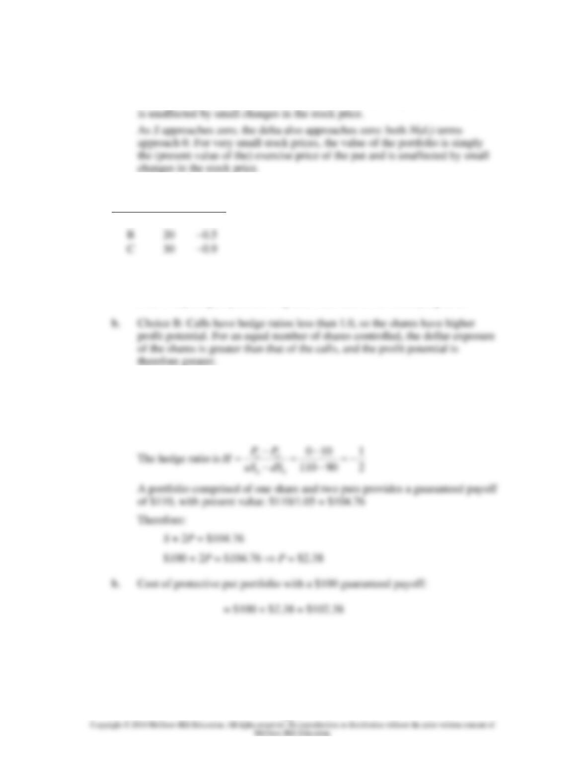
29. a. The delta of the collar is calculated as follows:
Position
Delta
Write call, X = $55
Chapter 21 – Option Valuation
21-7
b. If S becomes very large, then the delta of the collar approaches zero. Both
N(d1) terms approach 1. Intuitively, for very large stock prices, the value of
the portfolio is simply the (present value of the) exercise price of the call, and
30.
Put
X
Delta
A
10
−0.1
C
30
−0.9
31. a. Choice A: Calls have higher elasticity than shares. For equal dollar investments,
a call’s capital gain potential is greater than that of the underlying stock.
32. a. uS 0 = 110 Pu = 0
dS 0 = 90 Pd = 10
Chapter 21 – Option Valuation
21-8
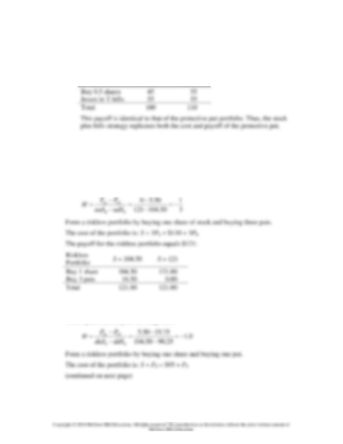
c. Our goal is a portfolio with the same exposure to the stock as the hypothetical
protective put portfolio. Since the put’s hedge ratio is –0.5, the portfolio
consists of (1 – 0.5) = 0.5 shares of stock, which costs $50, and the remaining
funds ($52.38) invested in T-bills, earning 5% interest.
Portfolio
S = 90
S = 110
33. The put values in the second period are:
Puu = 0
Pud = Pdu = 110 − 104.50 = 5.50
Pdd = 110 − 90.25 = 19.75
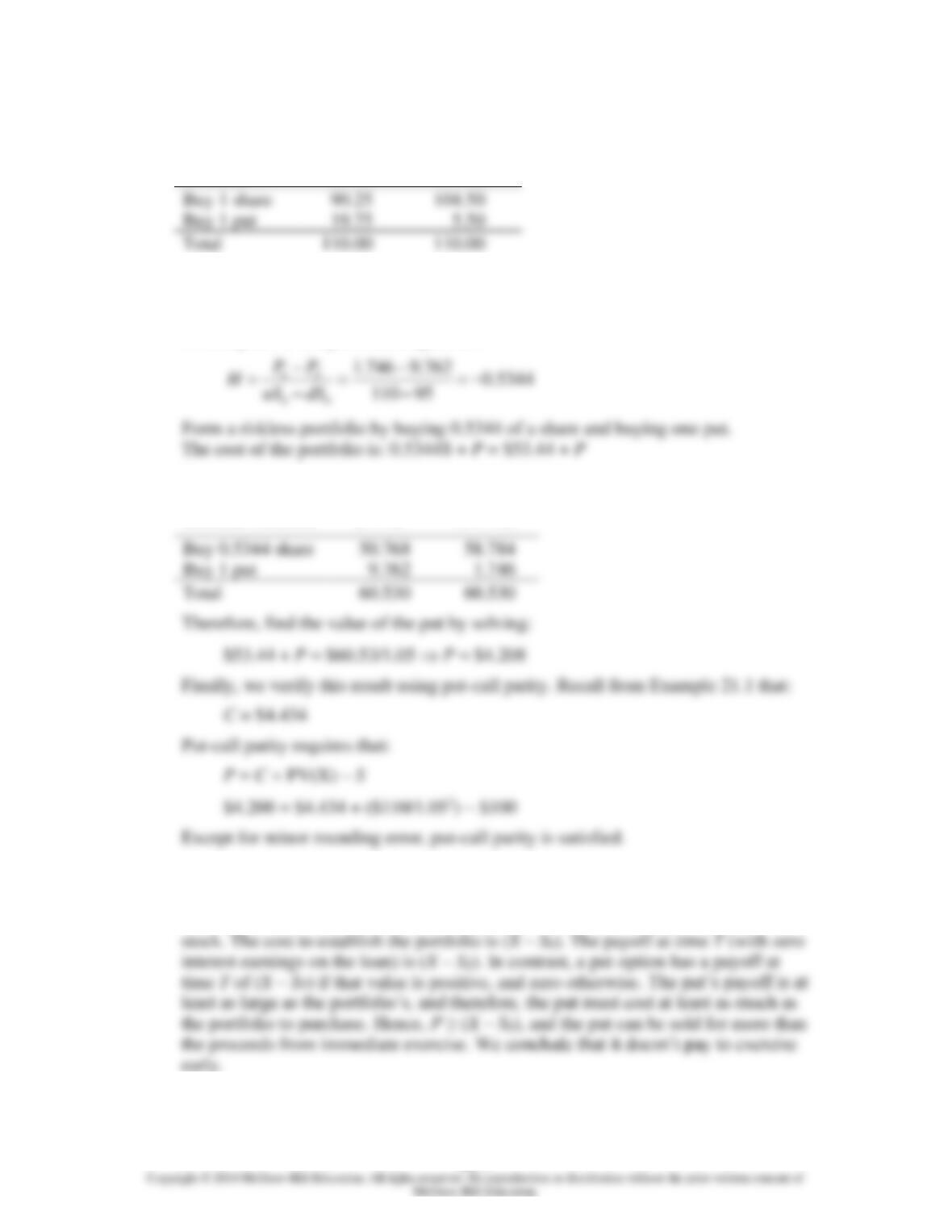
To compute Pu, first compute the hedge ratio:
Therefore, find the value of the put by solving:
$110 + 3Pu = $121/1.05 Pu = $1.746
To compute Pd , compute the hedge ratio:
Chapter 21 – Option Valuation
21-9
The payoff for the riskless portfolio equals $110:
Riskless
Portfolio
S = 90.25
S = 104.50
Therefore, find the value of the put by solving:
$95 + Pd = $110/1.05 Pd = $9.762
To compute P, compute the hedge ratio:
The payoff for the riskless portfolio equals $60.53:
Riskless Portfolio
S = 95
S = 110
34. If r = 0, then one should never exercise a put early. There is no “time value cost” to
waiting to exercise, but there is a “volatility benefit” from waiting. To show this
more rigorously, consider the following portfolio: lend $X and short one share of
Chapter 21 – Option Valuation
35. a. Xe−rT
b. X
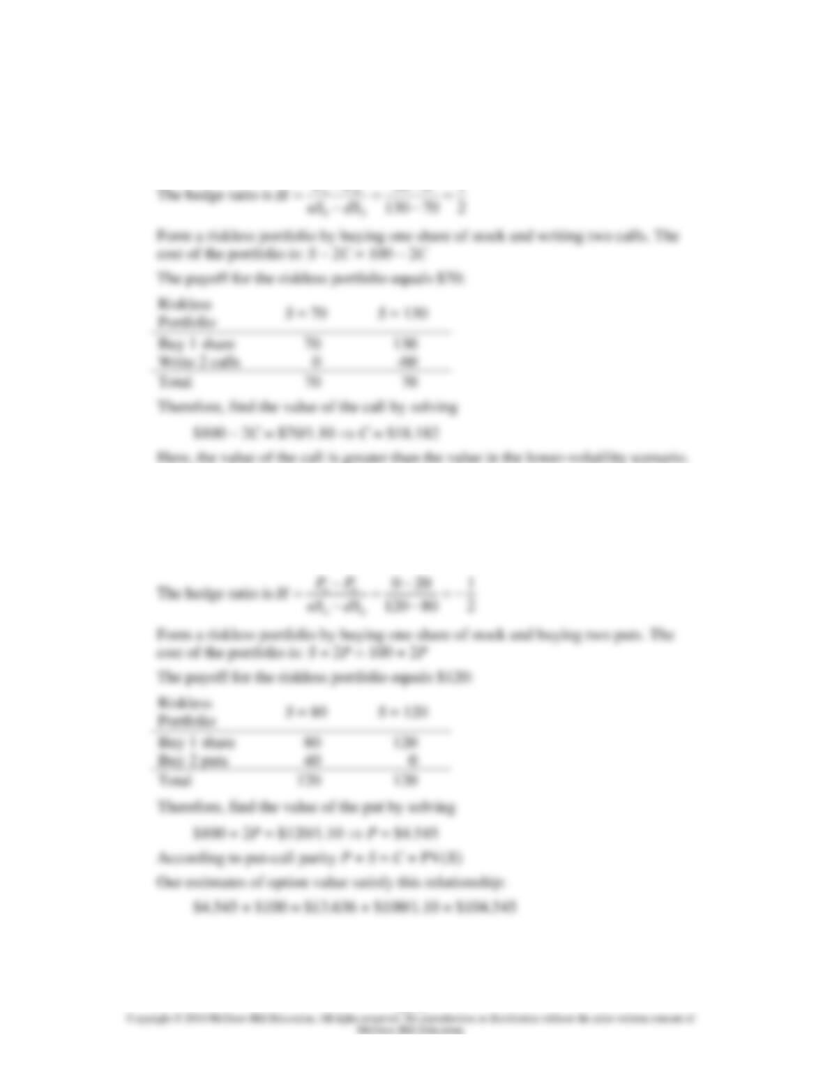
36. Step 1: Calculate the option values at expiration. The two possible stock prices and
the corresponding call values are:
uS 0 = 120 Cu = 20
dS 0 = 80 Cd = 0
Step 2: Calculate the hedge ratio.
Chapter 21 – Option Valuation
21–11
37. The two possible stock prices and the corresponding call values are:
uS 0 = 130 Cu = 30
dS 0 = 70 Cd = 0
38. The two possible stock prices and the corresponding put values are:
uS 0 = 120 Pu = 0
dS 0 = 80 Pd = 20
Chapter 21 – Option Valuation
39. If we assume that the only possible exercise date is just prior to the ex-dividend
date, then the relevant parameters for the Black-Scholes formula are:
S 0 = 60
r = 0.5% per month
40. True. The call option has an elasticity greater than 1.0. Therefore, the call’s
percentage rate of return is greater than that of the underlying stock. Hence the GM
41. False. The elasticity of a call option is higher the more out of the money is the
option. (Even though the delta of the call is lower, the value of the call is also
42. As the stock price increases, conversion becomes increasingly more assured. The
Chapter 21 – Option Valuation
21–13
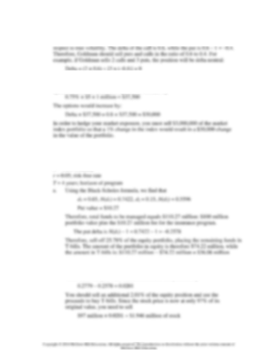
43. Goldman Sachs believes that the market assessment of volatility is too high. It
should sell options because the analysis suggests the options are overpriced with
44. If the stock market index increases 1%, the 1 million shares of stock on which the
options are written would be expected to increase by
45. S = 100; current value of portfolio
X = 100; floor promised to clients (0% return)
σ = 0.25; volatility
b. At the new portfolio value of 97, the put delta is
N(d1) – 1 = 0.7221 – 1 = –0.2779
This means that you must reduce the delta of the portfolio by
Chapter 21 – Option Valuation
21–14
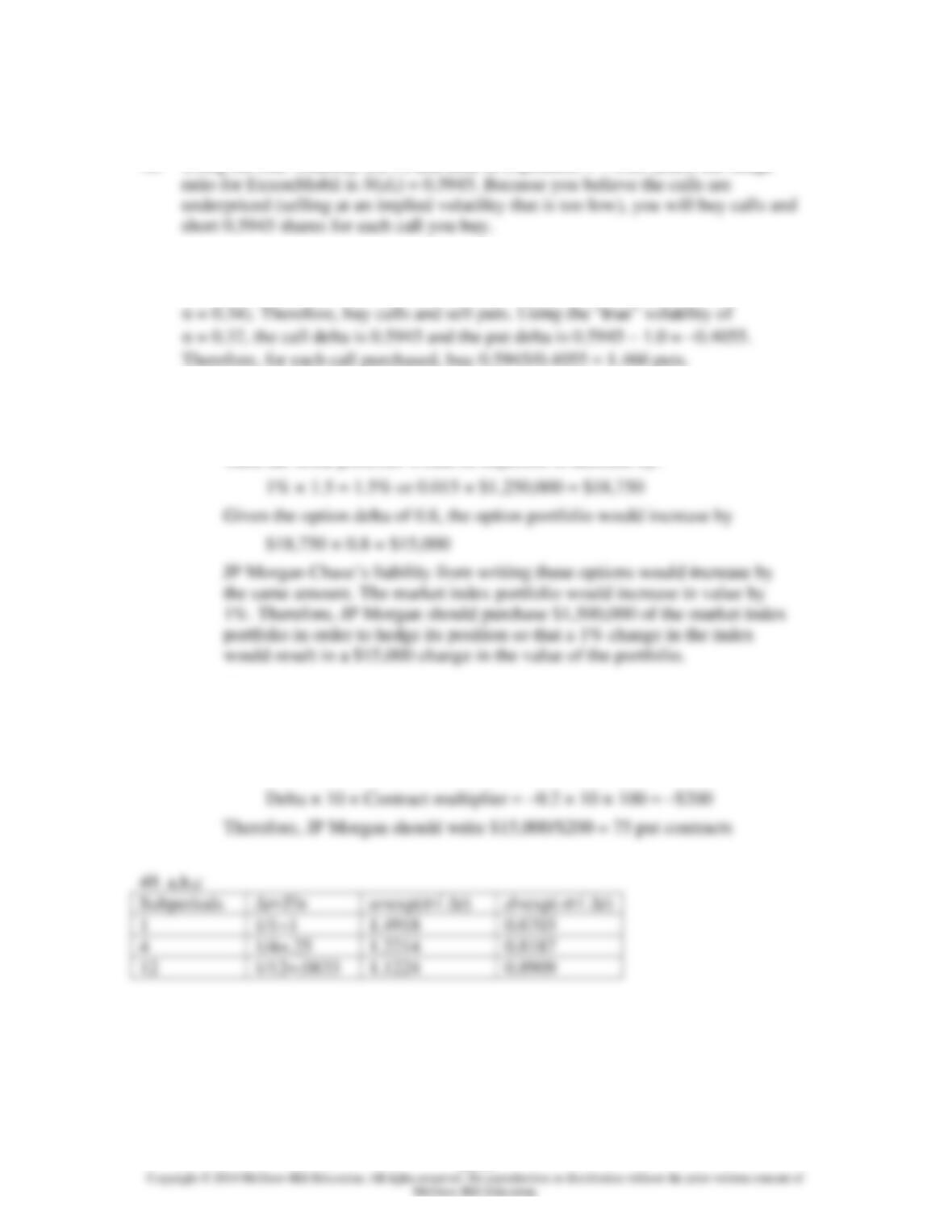
46. Using the true volatility (32%) and time to expiration T = 0.25 years, the hedge
47. The calls are cheap (implied σ = 0.30) and the puts are expensive (implied
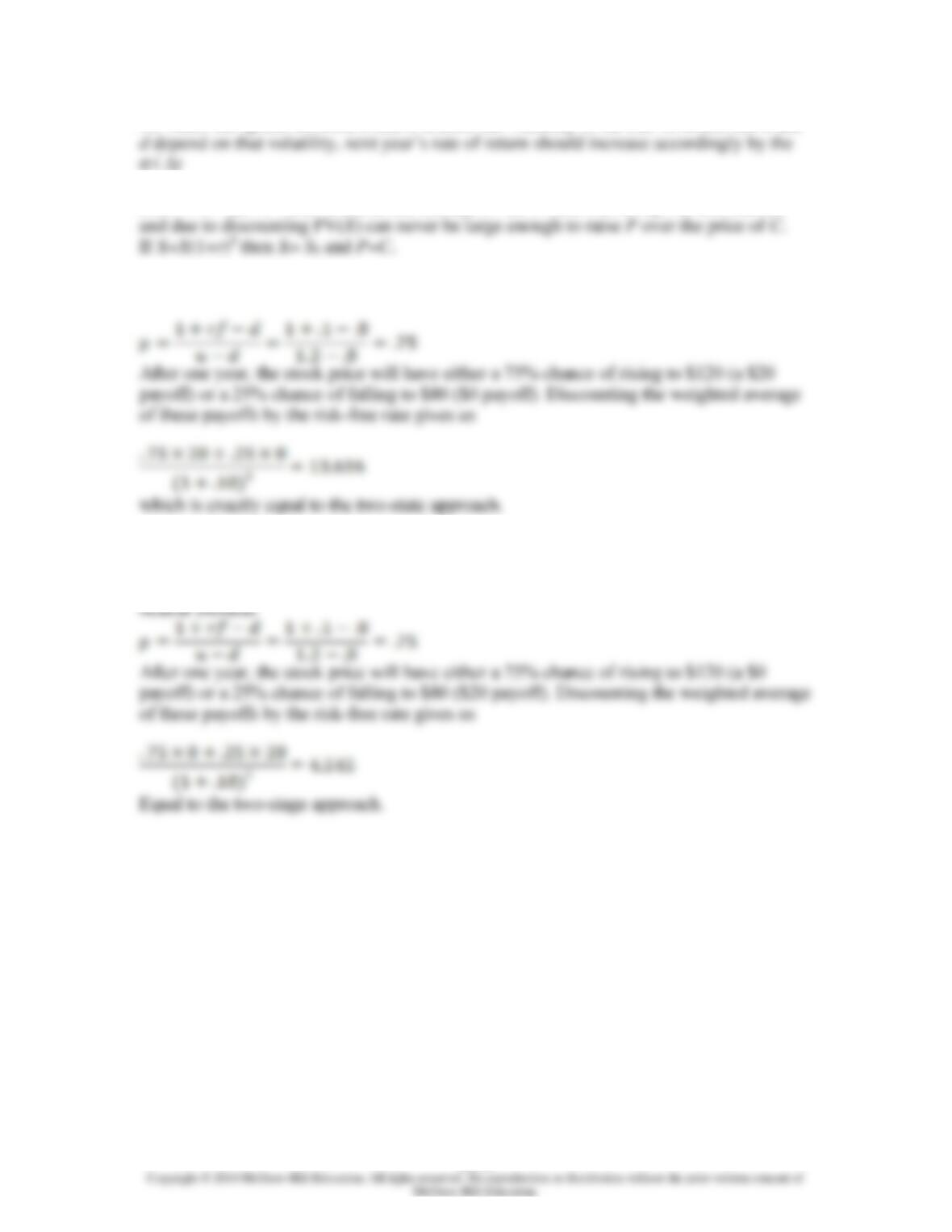
48. a. To calculate the hedge ratio, suppose that the market index increases by 1%.
Then the stock portfolio would be expected to increase by:
b. The delta of a put option is
0.8 – 1 = –0.2
Therefore, for every 1% the market increases, the index will rise by 10 points
and the value of the put option contract will change by
Chapter 21 – Option Valuation
21–15
50. Since the spread between u and d reflects the volatility of the rate of return and u and
51. P = C – S0 + PV(X). When at-the-money, X= S0. PV(X) will always be less than S0
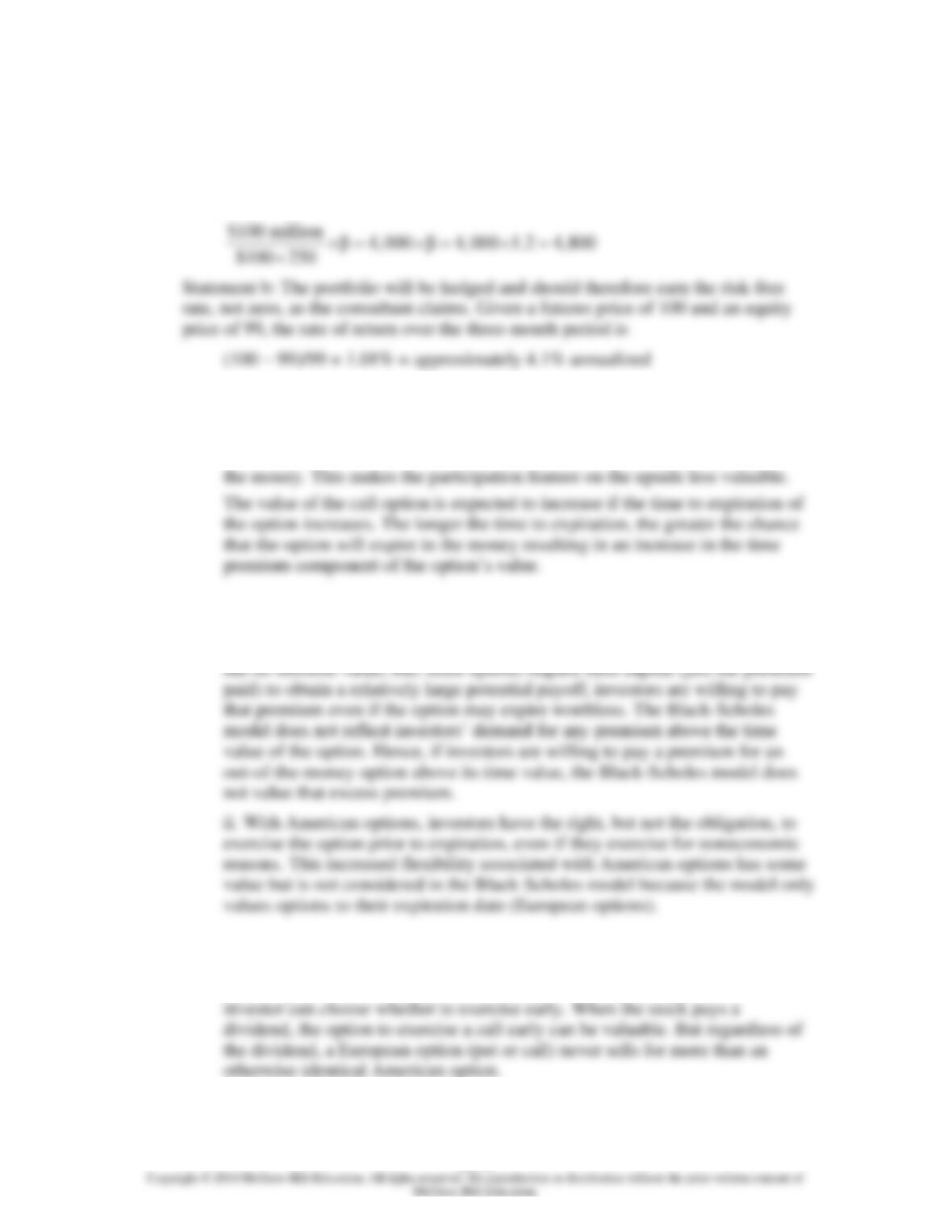
52. Using the risk-neutral shortcut, we must first calculate the risk-neutral probability p.
53. If the stock price rises, the payoff will be zero as profit from a put is only made when
the stock price is less than the exercise price. If the stock price falls, it falls below the
$100 exercise price and the payoff will be the difference between the two. Using the risk-
Chapter 21 – Option Valuation
21–16
CFA PROBLEMS
1. Statement a: The hedge ratio (determining the number of futures contracts to sell)
ought to be adjusted by the beta of the equity portfolio, which is 1.20. The correct
hedge ratio would be
2. a. The value of the call option decreases if underlying stock price volatility
decreases. The less volatile the underlying stock price, the less the chance of
extreme price movements—the lower the probability that the option expires in
b. i. When European options are out of the money, investors are essentially
saying that they are willing to pay a premium for the right, but not the
obligation, to buy or sell the underlying asset. The out-of-the-money option
3. a. American options should cost more (have a higher premium). American
options give the investor greater flexibility than European options since the
Chapter 21 – Option Valuation
21–17
b. C = S0 + P − PV(X) = $43 + $4 − $45/1.055 = $4.346
Note: we assume that Abaco does not pay any dividends.
c. i. An increase in short-term interest rate PV(exercise price) is lower, and
4. a. The two possible values of the index in the first period are:
uS0 = 1.20 × 50 = 60
dS0 = 0.80 × 50 = 40
The possible values of the index in the second period are:
uuS0 = (1.20)2 × 50 = 72
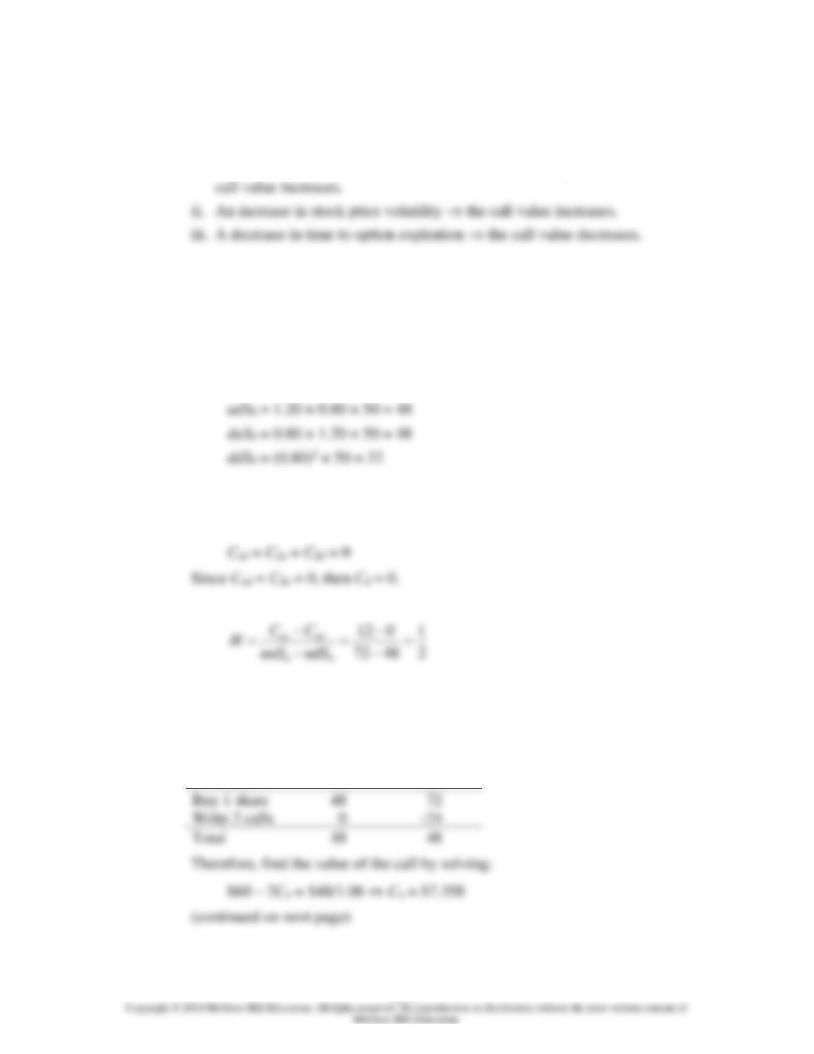
b. The call values in the second period are:
Cuu = 72 − 60 = 12
To compute Cu, first compute the hedge ratio:
Form a riskless portfolio by buying one share of stock and writing two calls.
The cost of the portfolio is: S – 2Cu = $60 – 2Cu
The payoff for the riskless portfolio equals $48:
Riskless
Portfolio
S = 48
S = 72
Chapter 21 – Option Valuation
21–18
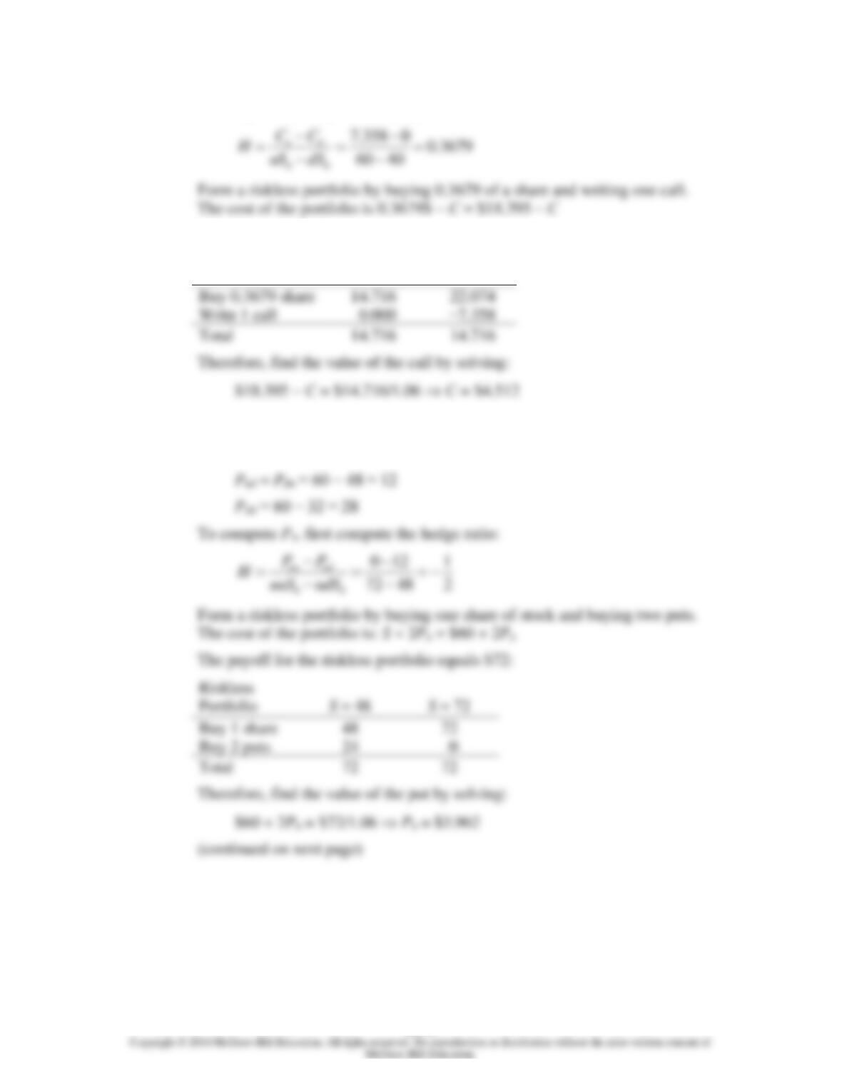
To compute C, compute the hedge ratio:
The payoff for the riskless portfolio equals $14.716:
Riskless Portfolio
S = 40
S = 60
c. The put values in the second period are:
Puu = 0
Chapter 21 – Option Valuation
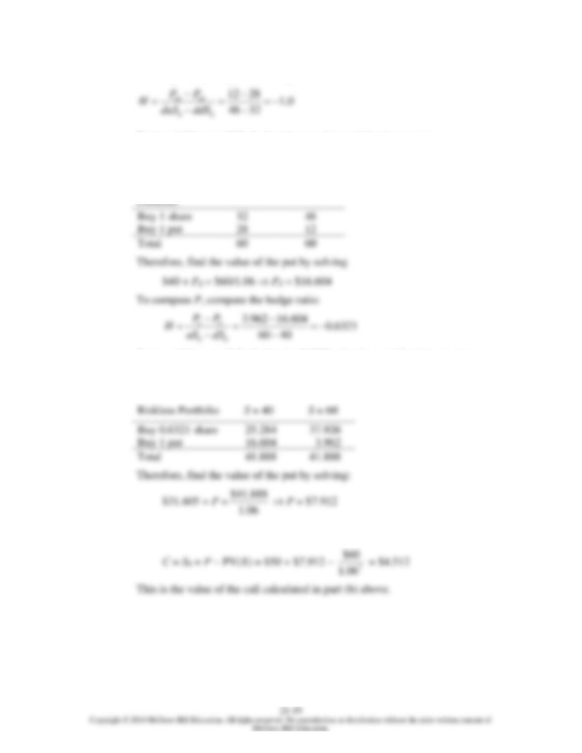
To compute Pd, compute the hedge ratio:
Form a riskless portfolio by buying one share and buying one put.
The cost of the portfolio is: S + Pd = $40 + Pd
The payoff for the riskless portfolio equals $60:
Riskless
S = 32
S = 48
Form a riskless portfolio by buying 0.6321 of a share and buying one put.
The cost of the portfolio is: 0.6321S + P = $31.605 + P
The payoff for the riskless portfolio equals $41.888:
d. According to put-call-parity:
Chapter 21 – Option Valuation
21–20
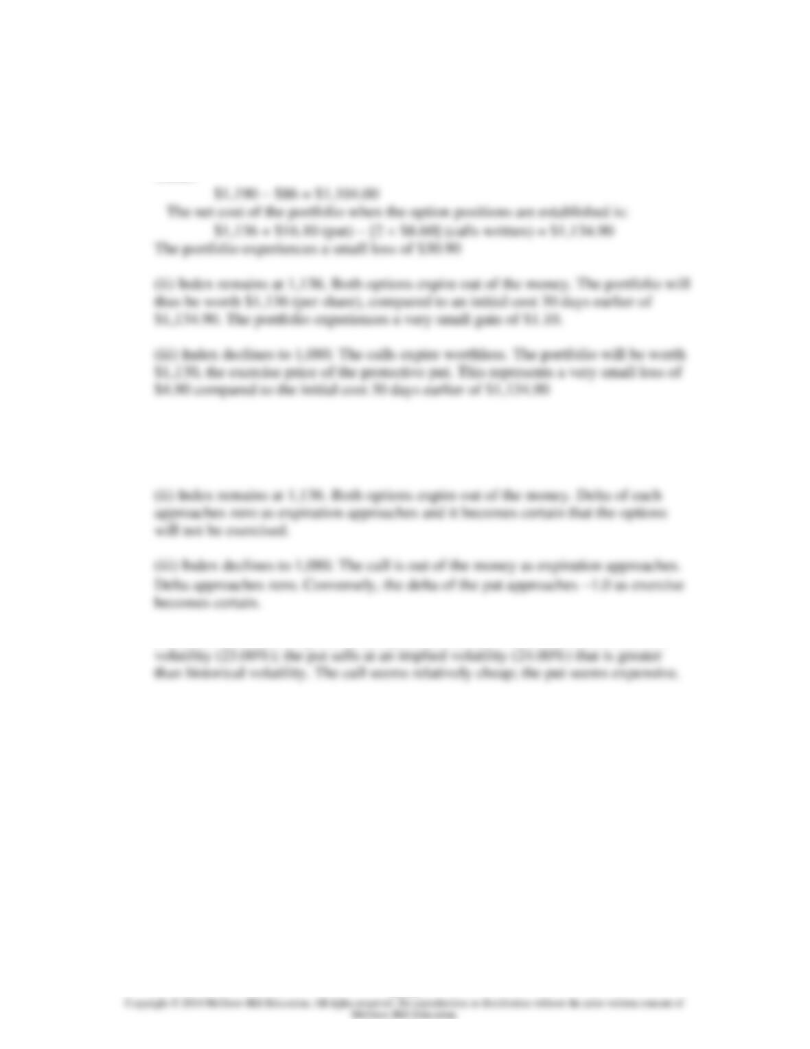
5. a. (i) Index increases to 1,193. The combined portfolio will suffer a loss. The written
calls expire in the money; the protective put purchased expires worthless. Let’s
analyze the outcome on a per-share basis. The payout for each call option is $43, for
a total cash outflow of $86. The stock is worth $1,190. The portfolio will thus be
worth:
b.(i) Index increases to 1,193. The delta of the call approaches 1.0 as the stock goes
deep into the money, while expiration of the call approaches and exercise becomes
essentially certain. The put delta approaches zero.
c. The call sells at an implied volatility (22.00%) that is less than recent historical