Chapter 20 – Options Markets: Introduction
20-1
CHAPTER 20: OPTIONS MARKETS: INTRODUCTION
PROBLEM SETS
1. Options provide numerous opportunities to modify the risk profile of a portfolio. The
simplest example of an option strategy that increases risk is investing in an ‘all options’
portfolio of at the money options (as illustrated in the text). The leverage provided by
2. Buying a put option on an existing portfolio provides portfolio insurance, which is
protection against a decline in the value of the portfolio. In the event of a decline in
3. An investor who writes a call on an existing portfolio takes a covered call position. If, at
expiration, the value of the portfolio exceeds the exercise price of the call, the writer of
Chapter 20 – Options Markets: Introduction
4. An option is out of the money when exercise of the option would be unprofitable. A call
option is out of the money when the market price of the underlying stock is less than the
exercise price of the option. If the stock price is substantially less than the exercise
price, then the likelihood that the option will be exercised is low, and fluctuations in the
market price of the stock have relatively little impact on the value of the option. This
sensitivity of the option price to changes in the price of the stock is called the option’s
delta, which is discussed in detail in Chapter 21. For options that are far out of the
money, delta is close to zero. Consequently, there is generally little to be gained or lost
5.
Cost
Payoff
Profit
a.
Call option, X = $100.00¤
$100.00¤$$100.00¤¤$$$100.
00====$100.00==$100.00¤
¤¤$100.000 ¤$$$1$$$100.00
$7.65
$5.00
-$2.65
b.
Put option, X = $100.00
$2.53
$0.00
-$2.53
c.
Call option, X = $105.00
$4.40
$0.00
-$4.40
d.
Put option, X = $105.00
$4.40
$0.00
-$4.40
e.
Call option, X = $110.00
$2.30
$0.00
-$2.30
f.
Put option, X = $110.00
$7.40
$5.00
-$2.40
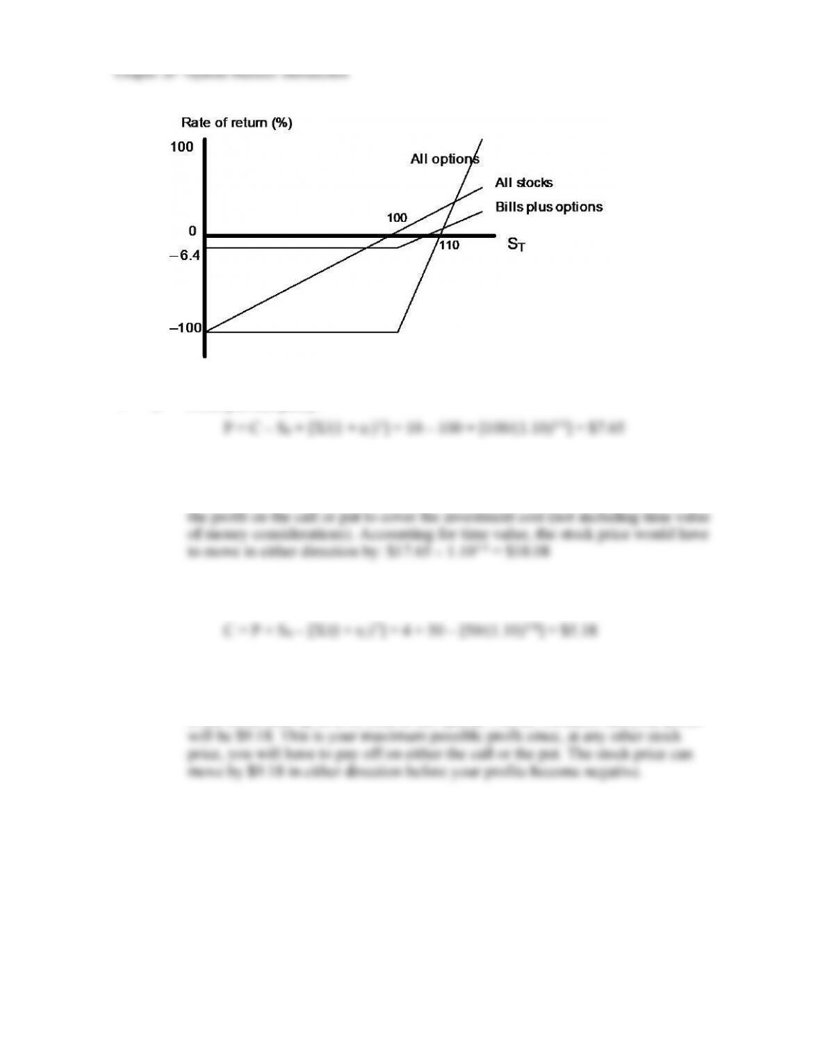
6. In terms of dollar returns, based on a $10,000 investment:
Price of Stock 6 Months from Now
Stock Price
$80
$100
$110
$120
All stocks (100 shares)
$8,000
$10,000
$11,000
$12,000
All options (1,000 options)
$0
$0
$10,000
$20,000
Bills + 100 options
$9,360
$9,360
$10,360
$11,360
In terms of rate of return, based on a $10,000 investment:
Price of Stock 6 Months from Now
Stock Price
$80
$100
$110
$120
All stocks (100 shares)
-20%
0%
10%
20%
All options (1,000 options)
-100%
-100%
0%
100%
Bills + 100 options
-6.4%
-6.4%
3.6%
13.6%
20-3
7. a. From put-call parity:
b. Purchase a straddle, i.e., both a put and a call on the stock. The total cost of the
straddle is: $10 + $7.65 = $17.65
This is the amount by which the stock would have to move in either direction for
8. a. From put-call parity:
b. Sell a straddle, i.e., sell a call and a put to realize premium income of:
$5.18 + $4 = $9.18
If the stock ends up at $50, both of the options will be worthless and your profit
Chapter 20 – Options Markets: Introduction
20-4
c. Buy the call, sell (write) the put, lend: $50/(1.10)1/4
The payoff is as follows:
Position
Immediate CF
CF in 3 months
S T ≤ X
S T > X
Call (long)
C = 5.18
0
S T – 50
Put (short)
–P = 4.00
– (50 – S T)
0
Lending position
82.48
10.1
50
4/1 =
50
50
Total
C – P +
00.50
10.1
50
4/1 =
S T
S T
By the put-call parity theorem, the initial outlay equals the stock price:
9. a.
Outcome
S T ≤ X
S T > X
Stock
S T + D
S T + D
Put
X – S T
0
Total
X + D
S T + D
b.
Outcome
S T ≤ X
S T > X
Call
0
ST – X
Zeros
X + D
X + D
Total
X + D
ST + D
The total payoffs for the two strategies are equal regardless of whether S T exceeds
X.
c. The cost of establishing the stock-plus-put portfolio is: S0 + P
The cost of establishing the call-plus-zero portfolio is: C + PV(X + D)
Therefore:
Chapter 20 – Options Markets: Introduction
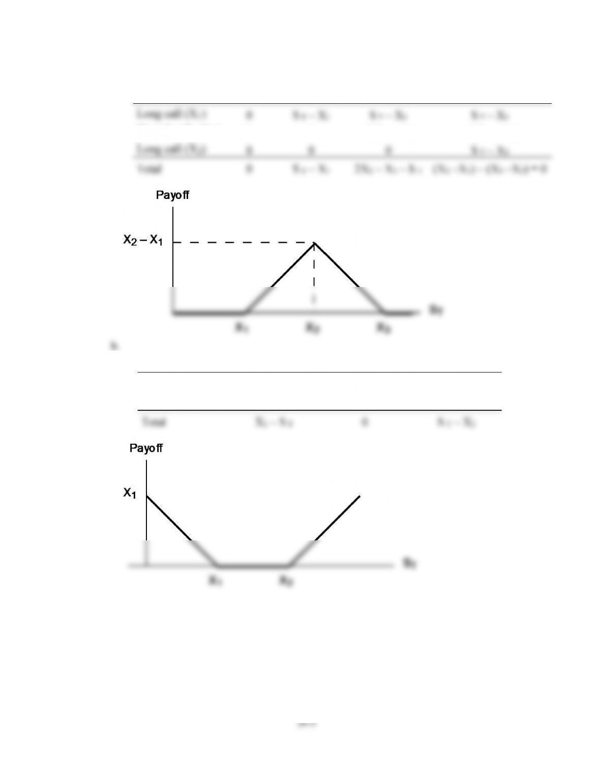
10. a.
Position
S T < X1
X1 S T X2
X2 < S T X3
X3 < S T
Long call (X1)
0
S T – X1
S T – X1
S T – X1
Short 2 calls (X2)
0
0
–2(S T – X2)
–2(S T – X2)
Long call (X3)
0
0
0
S T – X3
Total
0
S T – X1
2X2 – X1 – S T
(X2 –X1) – (X3 –X2) = 0
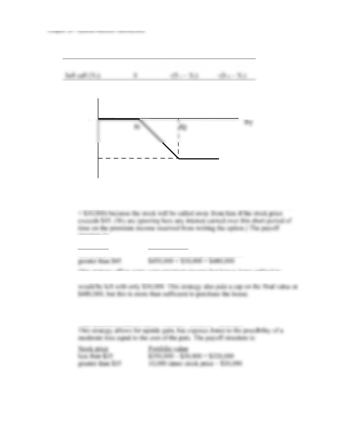
b.
Position
S T < X1
X1 S T X2
X2X2XX2
X2X2X2X2
X2 < S T
Buy call (X2)
0
0
S T – X2
Buy put (X1)
X1 – S T
0
0
Total
X1 – S T
0
S T – X2
20-6
11.
Position
S T < X1
X1 S T X2
XX2
X2 < S T
Buy call (X2)
0
0
S T – X2
Sell call (X1)
0
–(S T – X1)
–(S T – X1)
Total
0
X1 – S T
X1 – X2
Payoff
0
S
T
X
1
X
2
Payoff
–(X
2
–
X
1
)
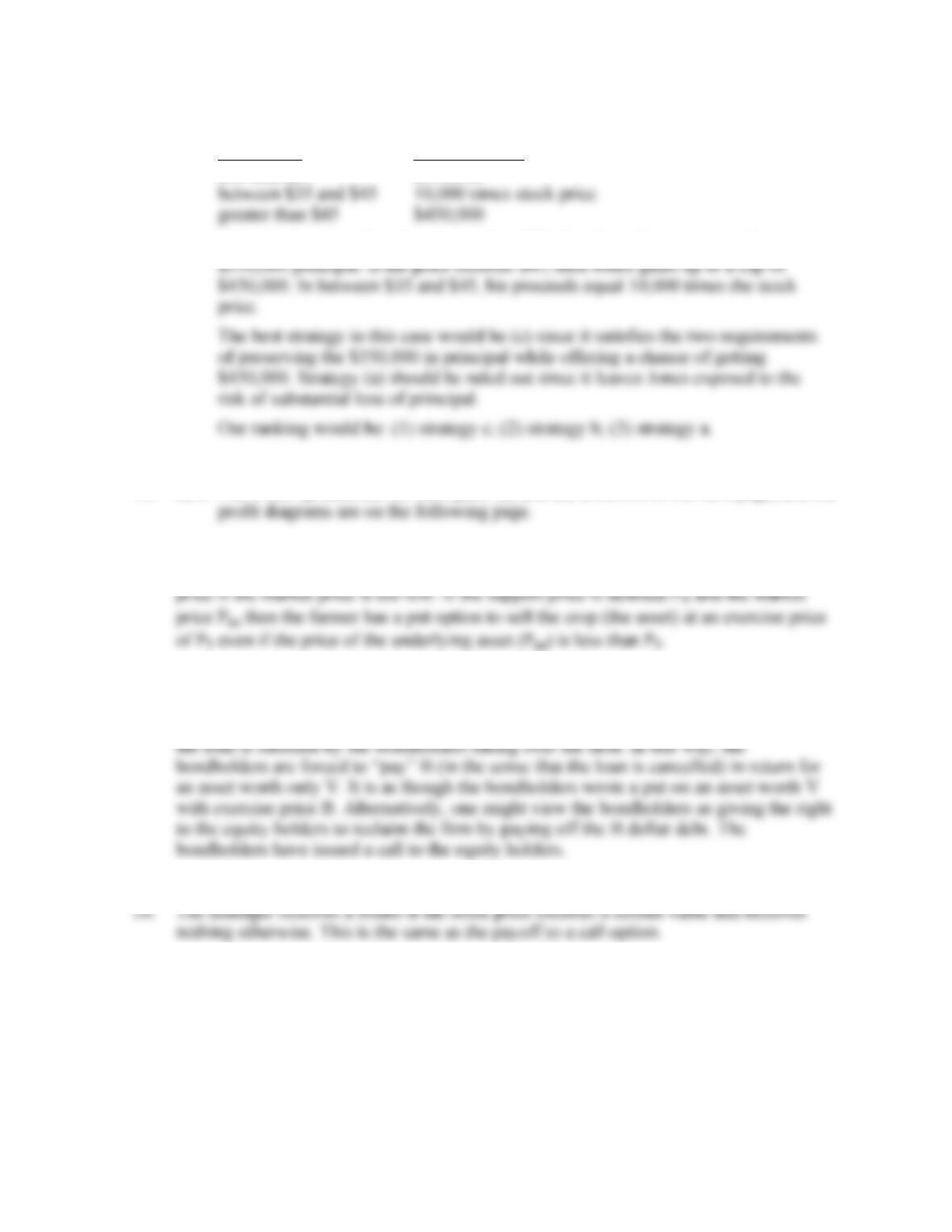
12. a. By writing covered call options, Jones receives premium income of $30,000. If, in
January, the price of the stock is less than or equal to $45, then Jones will have his
stock plus the premium income. But the most he can have at that time is ($450,000
structure is:
Stock price Portfolio value
less than $45 10,000 times stock price + $30,000
This strategy offers some extra premium income but leaves Jones subject to
substantial downside risk. At an extreme, if the stock price fell to zero, Jones
b. By buying put options with a $35 strike price, Jones will be paying $30,000 in
premiums in order to insure a minimum level for the final value of his position.
That minimum value is: ($35 10,000) – $30,000 = $320,000
Chapter 20 – Options Markets: Introduction
20-7
c. The net cost of the collar is zero. The value of the portfolio will be as follows:
Stock price Portfolio value
less than $35 $350,000
If the stock price is less than or equal to $35, then the collar preserves the
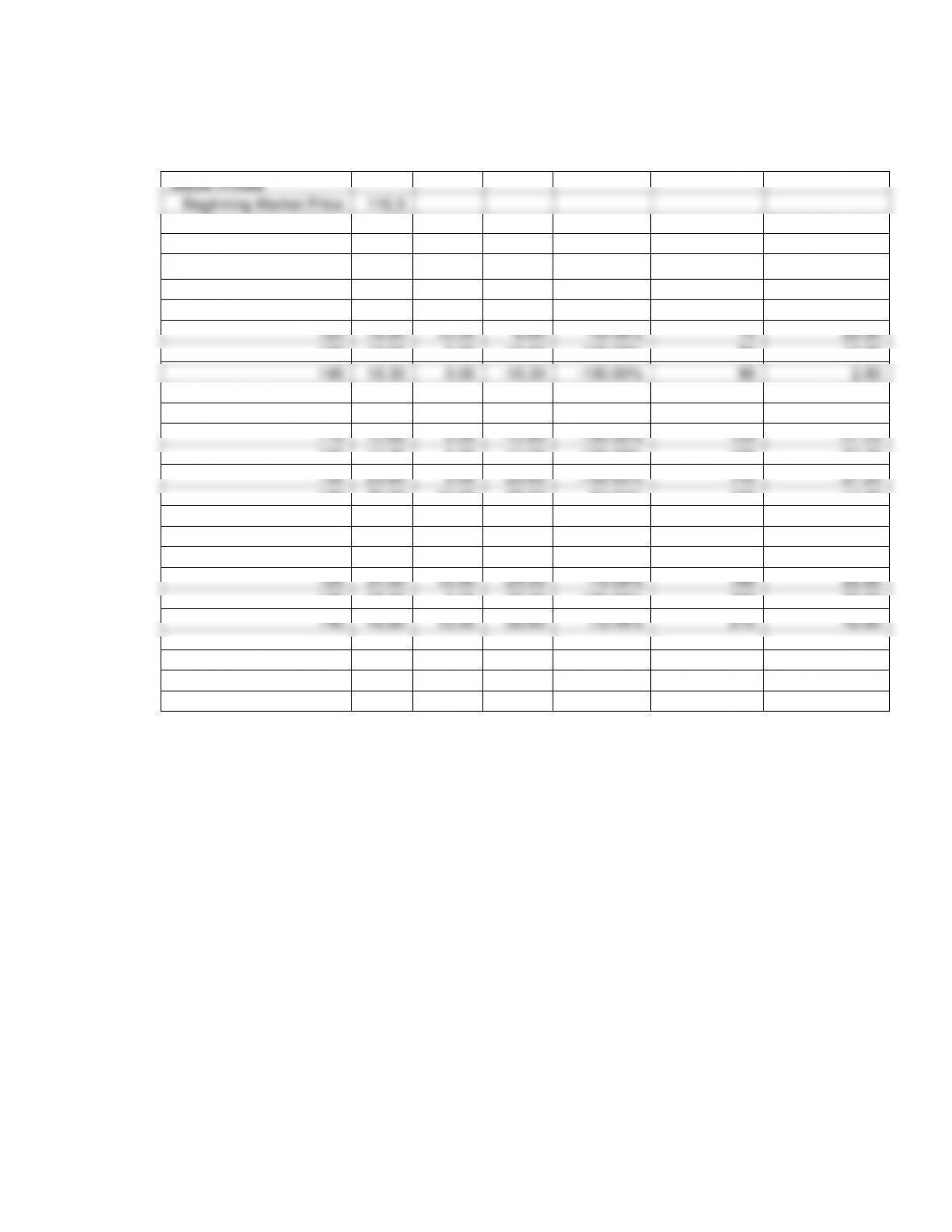
13. a., b. The Excel spreadsheet for both parts (a) and (b) is shown on the next page, and the
14. The farmer has the option to sell the crop to the government for a guaranteed minimum
15. The bondholders have, in effect, made a loan which requires repayment of B dollars,
where B is the face value of bonds. If, however, the value of the firm (V) is less than B,
Chapter 20 – Options Markets: Introduction
20-8
Spreadsheet for Problem 13:
Stock Prices
Beginning Market Price
116.5
Ending Market Price
130
X 130 Straddle
Ending
Profit
Buying Options:
Stock Price
–37.20
Call Options Strike
Price
Payoff
Profit
Return %
50
42.80
110
22.80
20.00
–2.80
–12.28%
60
32.80
120
16.80
10.00
–6.80
–40.48%
70
22.80
130
13.60
0.00
–13.60
-100.00%
80
12.80
140
10.30
0.00
–10.30
-100.00%
90
2.80
100
–7.20
Put Options Strike
Price
Payoff
Profit
Return %
110
–17.20
110
12.60
0.00
–12.60
-100.00%
120
–27.20
120
17.20
0.00
–17.20
-100.00%
130
–37.20
130
23.60
0.00
–23.60
-100.00%
140
–27.20
140
30.50
10.00
–20.50
–67.21%
150
–17.20
160
–7.20
Straddle
Price
Payoff
Profit
Return %
170
2.80
110
35.40
20.00
–15.40
–43.50%
180
12.80
120
34.00
10.00
–24.00
–70.59%
190
22.80
130
37.20
0.00
–37.20
-100.00%
200
32.80
140
40.80
10.00
–30.80
-75.49%
210
42.80
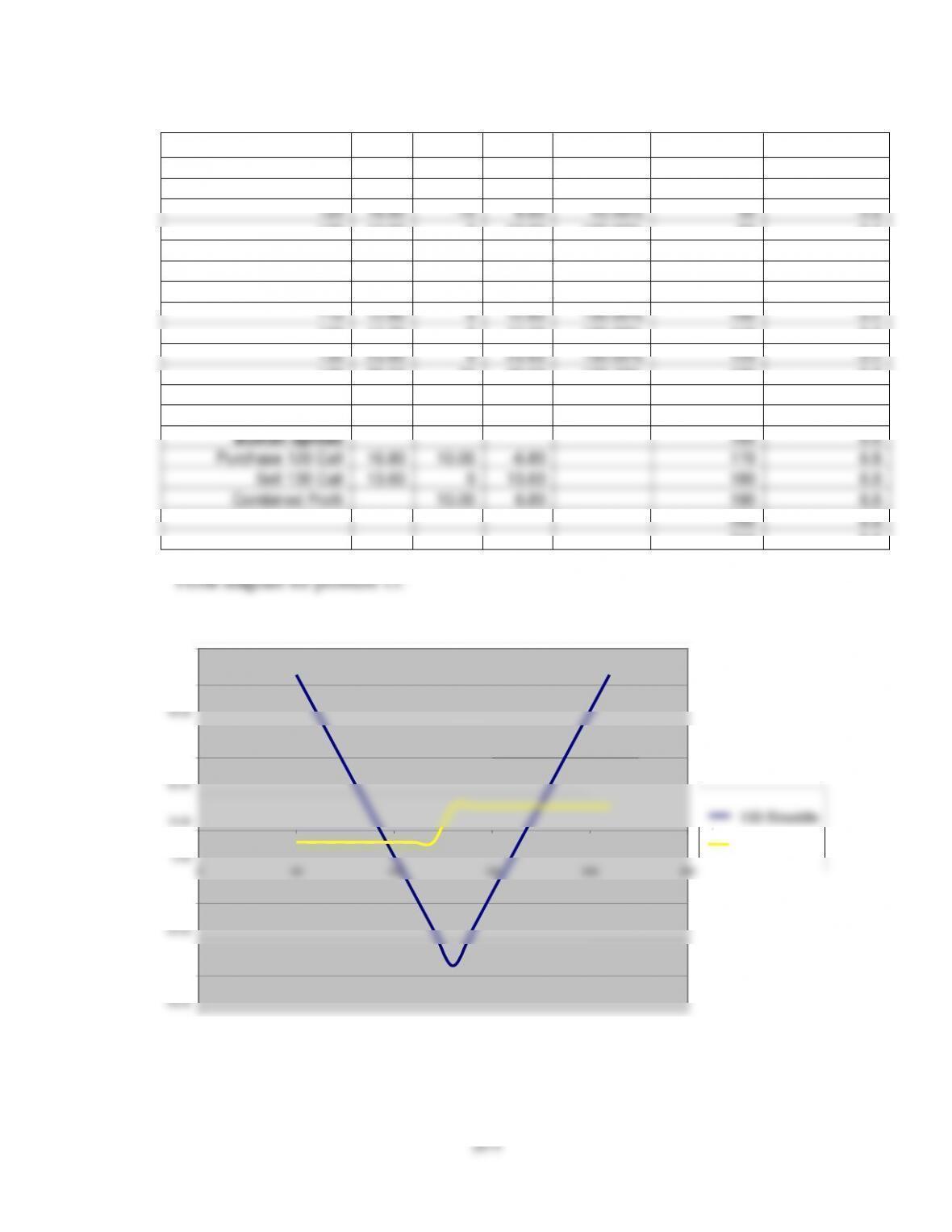
Chapter 20 – Options Markets: Introduction
Selling Options:
Bullish
Call Options Strike
Price
Payoff
Profit
Return %
Ending
Spread
110
22.80
–20
2.80
12.28%
Stock Price
6.80
120
16.80
–10
6.80
40.48%
50
–3.2
130
13.60
0
13.60
100.00%
60
-3.2
140
10.30
0
10.30
100.00%
70
–3.2
80
–3.2
Put Options Strike
Price
Payoff
Profit
Return %
90
–3.2
110
12.60
0
12.60
100.00%
100
–3.2
120
17.20
0
17.20
100.00%
110
–3.2
130
23.60
0
23.60
100.00%
120
–3.2
140
30.50
10
40.50
132.79%
130
6.8
140
6.8
Money Spread
Price
Payoff
Profit
150
6.8
Bullish Spread
160
6.8
Purchase 120 Call
16.80
10.00
–6.80
170
6.8
Sell 130 Call
13.60
0
13.60
180
6.8
Combined Profit
10.00
6.80
190
6.8
200
6.8
210
6.8
Spreads and Straddles
-50.00
-40.00
-30.00
-20.00
-10.00
0.00
10.00
20.00
30.00
40.00
50.00
0
50
100
150
200
250
Stock Price
130 Straddle
Bullish Spread
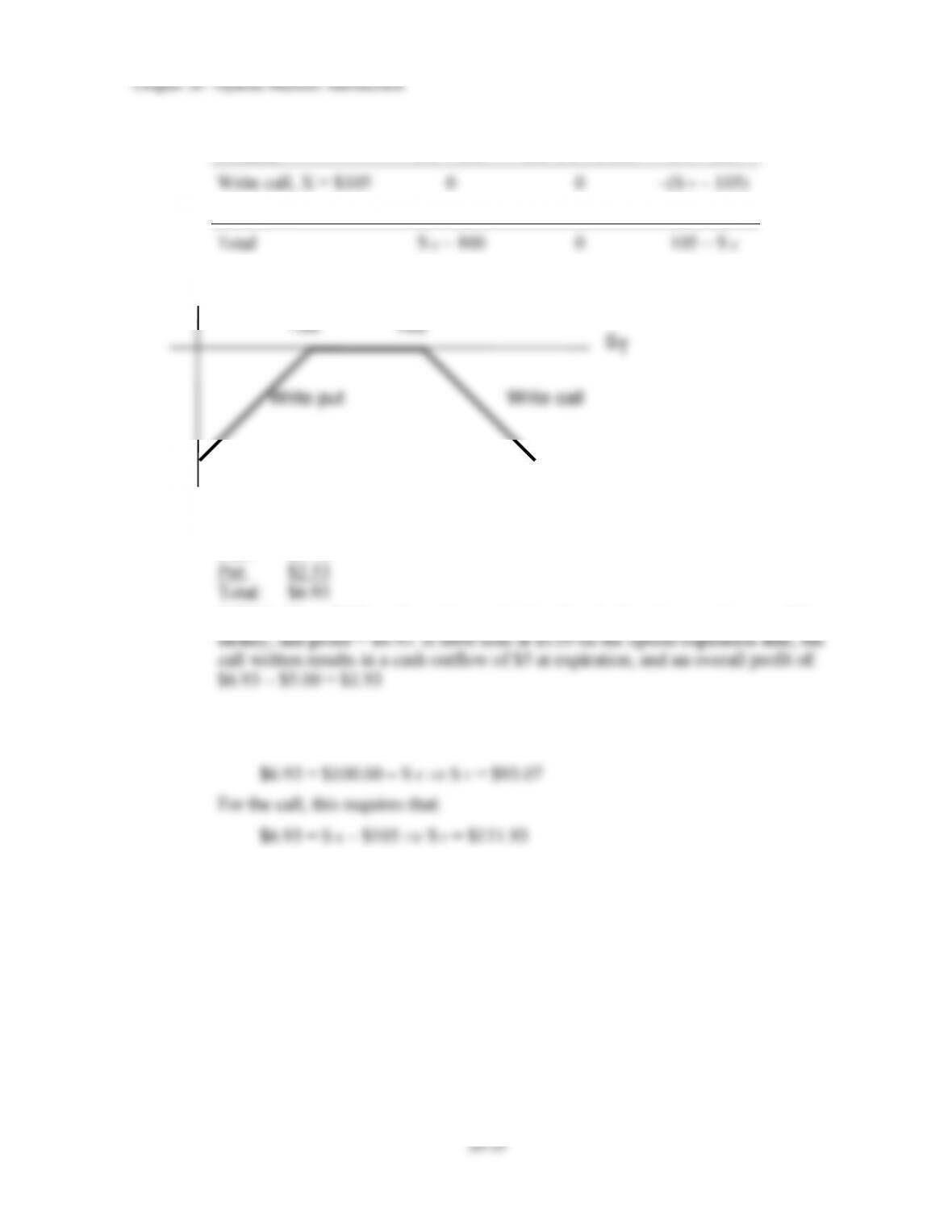
20–11
18. The put with the higher exercise price must cost more. Therefore, the net outlay to
establish the portfolio is positive.
Position
S T < 90
90 S T 95
S T > 95
Write put, X = $90
–(90 – S T)
0
0
Buy put, X = $95
95 – S T
95 – S T
0
Total
5
95 – S T
0
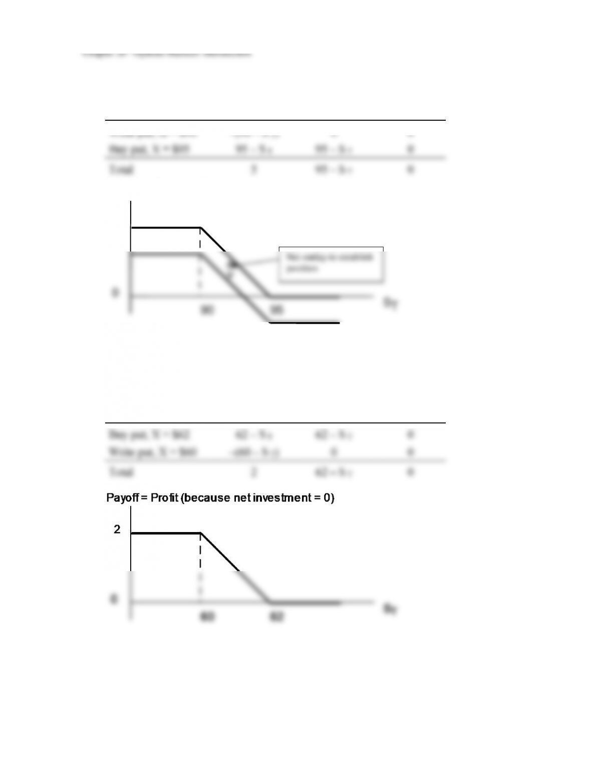
The payoff and profit diagram is:
0
S
T
Payoff
5
90
95
Profit
Net outlay to establish
position
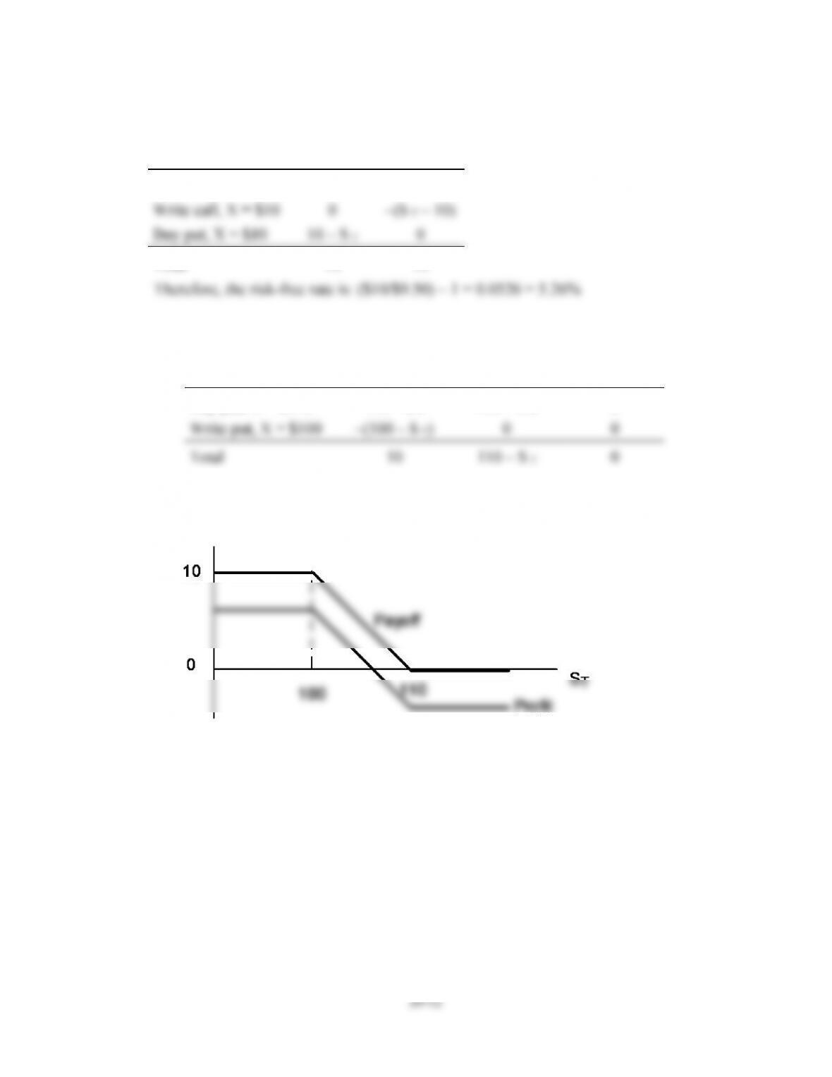
19. Buy the X = 62 put (which should cost more but does not) and write the X = 60 put.
Since the options have the same price, your net outlay is zero. Your proceeds at
expiration may be positive, but cannot be negative.
Position
S T < 60
60 S T 62
S T > 62
Buy put, X = $62
62 – S T
62 – S T
0
Write put, X = $60
–(60 – S T)
0
0
Total
2
62 – S T
0
Chapter 20 – Options Markets: Introduction
20. The following payoff table shows that the portfolio is riskless with time-T value equal to
$10:
Position
S T ≤ 10
S T > 10
Buy stock
S T
S T
Write call, X = $10
0
–(S T – 10)
Buy put, X = $10
10 – S T
0
Total
10
10
21. a., b.
Position
S T < 100
100 S T 110
S T > 110
Buy put, X = $110
110 – S T
110 – S T
0
Write put, X = $100
–(100 – S T)
0
0
Total
10
110 – S T
0
The net outlay to establish this position is positive. The put you buy has a higher
exercise price than the put you write, and therefore must cost more than the put
that you write. Therefore, net profits will be less than the payoff at time T.
c. The value of this portfolio generally decreases with the stock price. Therefore, its
beta is negative.
20–13
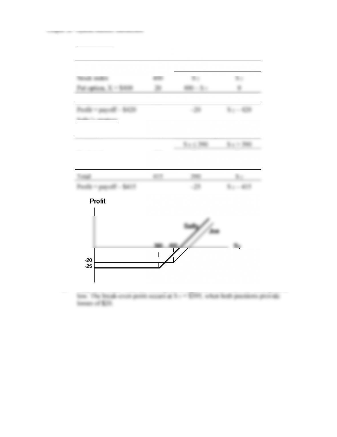
22. a. Joe’s strategy
Position
Cost
Payoff
S T 400
S T > 400
Stock index
400
S T
S T
Put option, X = $400
20
400 – S T
0
Total
420
400
S T
Profit = payoff – $420
–20
S T – 420
Sally’s strategy
Position
Cost
Payoff
S T 390
S T > 390
Stock index
400
S T
S T
Put option, X = $390
15
390 – S T
0
Total
415
390
S T
Profit = payoff – $415
–25
S T – 415
b. Sally does better when the stock price is high, but worse when the stock price is
c. Sally’s strategy has greater systematic risk. Profits are more sensitive to the value of
the stock index.
Chapter 20 – Options Markets: Introduction
23. a., b. (See graph below)
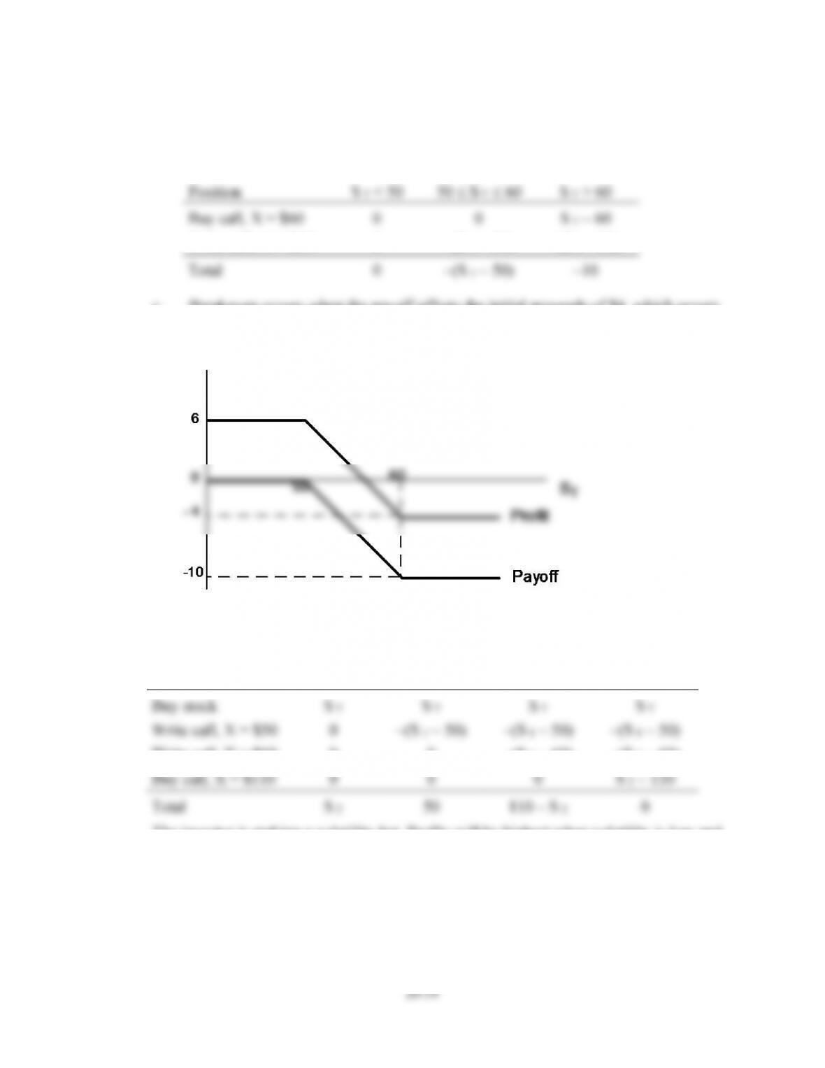
This strategy is a bear spread. Initial proceeds = $9 – $3 = $6
The payoff is either negative or zero:
Position
S T < 50
50 S T 60
S T > 60
Buy call, X = $60
0
0
S T – 60
Write call, X = $50
0
–(S T – 50)
–(S T – 50)
Total
0
–(S T – 50)
–10
c. Breakeven occurs when the payoff offsets the initial proceeds of $6, which occurs
at stock price S T = $56. The investor must be bearish: the position does worse
when the stock price increases.
24. Buy a share of stock, write a call with X = $50, write a call with X = $60, and buy a call
with X = $110.
Position
S T < 50
50 S T 60
60 < S T 110
S T > 110
Buy stock
S T
S T
S T
S T
Write call, X = $50
0
–(S T – 50)
–(S T – 50)
–(S T – 50)
Write call, X = $60
0
0
–(S T – 60)
–(S T – 60)
Buy call, X = $110
0
0
0
S T – 110
Total
S T
50
110 – S T
0
The investor is making a volatility bet. Profits will be highest when volatility is low and
the stock price S T is between $50 and $60.
20–15
25. a.
Position
S T ≤ 780
S T > 780
Buy stock
S T
S T
Buy put
780 – S T
0
Total
780
S T
Position
S T ≤ 840
S T > 840
Buy call
0
S T – 840
Buy T-bills
840
840
Total
840
S T
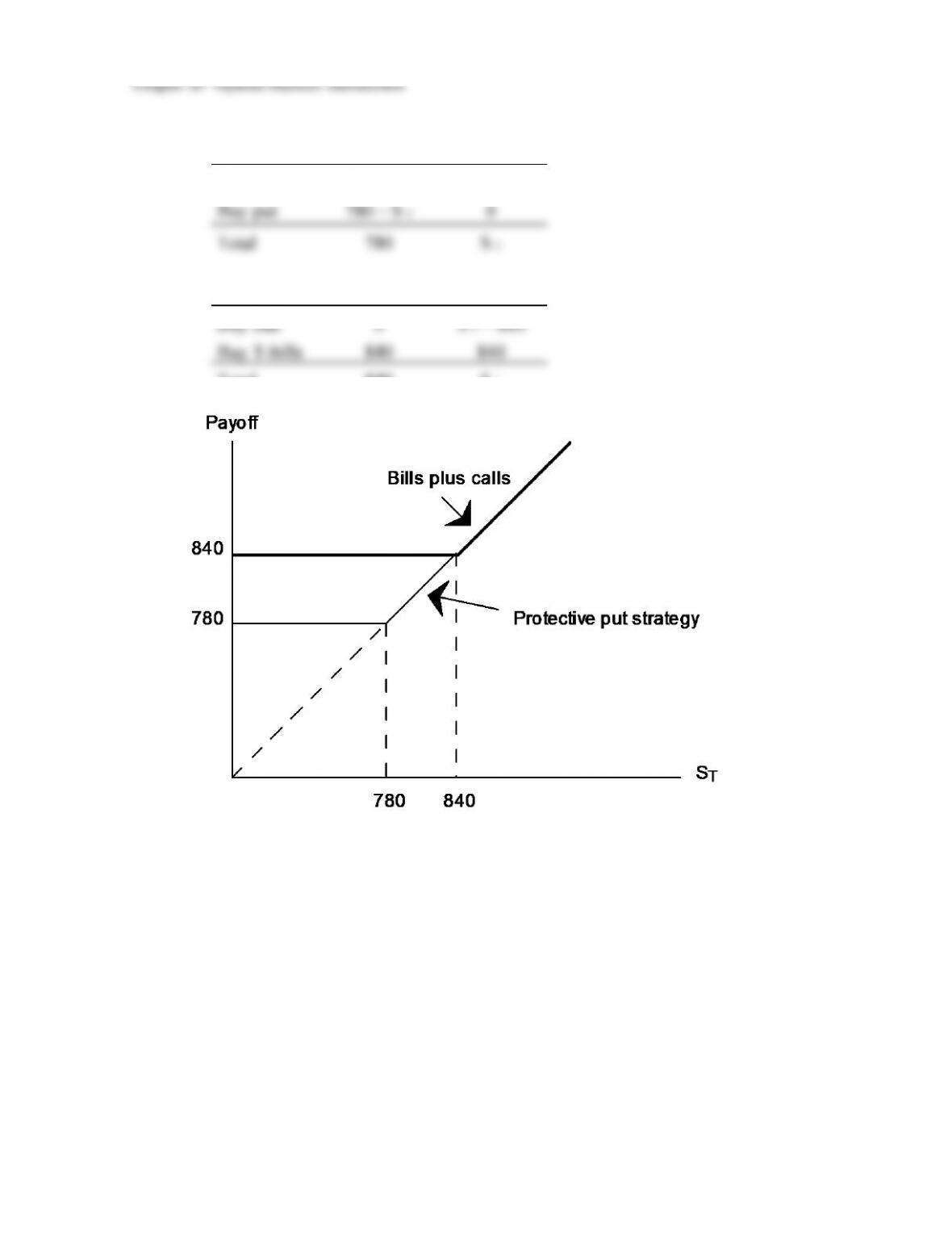
b. The bills plus call strategy has a greater payoff for some values of S T and never a
lower payoff. Since its payoffs are always at least as attractive and sometimes
greater, it must be more costly to purchase.
Chapter 20 – Options Markets: Introduction
20–16
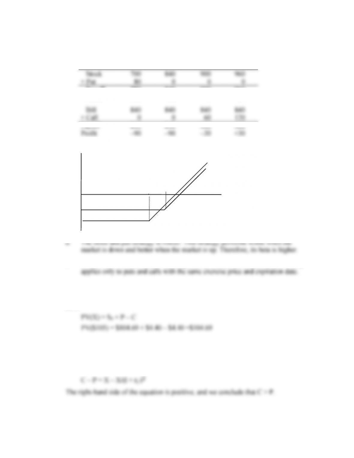
c. The initial cost of the stock plus put position is: $900 + $6 = $906
The initial cost of the bills plus call position is: $810 + $120 = $930
S T = 700
S T = 840
S T = 900
S T = 960
Stock
700
840
900
960
+ Put
80
0
0
0
Payoff
780
840
900
960
Profit
–126
–66
–6
54
Bill
840
840
840
840
+ Call
0
0
60
120
Payoff
840
840
900
960
Profit
–90
–90
–30
+30
Profit
Bills plus calls
Protective put
–90
–126
780
840
S
T
e. Parity is not violated because these options have different exercise prices. Parity
26. According to put-call parity (assuming no dividends), the present value of a payment of
$105 can be calculated using the options with February expiration and exercise price of
$105.
27. From put-call parity:
C – P = S0 – X/(l + rf )T
If the options are at the money, then S0 = X and:
Chapter 20 – Options Markets: Introduction
20–17
CFA PROBLEMS
1. a. Donie should choose the long strangle strategy. A long strangle option strategy
consists of buying a put and a call with the same expiration date and the same
underlying asset, but different exercise prices. In a strangle strategy, the call has an
exercise price above the stock price and the put has an exercise price below the
stock price. An investor who buys (goes long) a strangle expects that the price of
b. i. The maximum possible loss per share is $9.00, which is the total cost of the two
options ($5.00 + $4.00).
ii. The maximum possible gain is unlimited if the stock price moves outside the
breakeven range of prices.
2. i. Equity index-linked note: Unlike traditional debt securities that pay a scheduled
rate of coupon interest on a periodic basis and the par amount of principal at
ii. Commodity-linked bear bond: Unlike traditional debt securities that pay a
scheduled rate of coupon interest on a periodic basis and the par amount of
principal at maturity, the commodity-linked bear bond allows an investor to
Chapter 20 – Options Markets: Introduction
20–18
3. i. Conversion value of a convertible bond is the value of the security if it is
converted immediately. That is:
Conversion value =
ii. Market conversion price is the price that an investor effectively pays for the
common stock if the convertible bond is purchased:
Market conversion price =
4. a. i. The current market conversion price is computed as follows:
Market conversion price =
ii. The expected one-year return for the Ytel convertible bond is:
Expected return = [(end of year price + coupon)/current price] – 1
iii. The expected one-year return for the Ytel common equity is:
b. The two components of a convertible bond’s value are:
• the straight bond value, which is the convertible bond’s value as a bond, and;
(i.) In response to the increase in Ytel’s common equity price, the straight bond
value should stay the same and the option value should increase.
The increase in equity price does not affect the straight bond value component of
Chapter 20 – Options Markets: Introduction
(ii.) In response to the increase in interest rates, the straight bond value should
decrease and the option value should increase.