Investments & Securities Chapter 17 Analysis Bonds With Embedded Options Summary This Look How

CHAPTER 17

ANALYSIS OF BONDS WITH EMBEDDED OPTIONS

CHAPTER SUMMARY

In this chapter we look at how to analyze bonds with embedded options. Because the most

common type of option embedded in a bond is a call option, our primary focus is on callable

bonds. We begin by looking at the limitations of traditional yield spread analysis. Although

corporate bonds are used in our examples, the analysis presented in this chapter is equally

applicable to agency securities and municipal securities.

DRAWBACKS OF TRADITIONAL YIELD SPREAD ANALYSIS

STATIC SPREAD: AN ALTERNATIVE TO YIELD SPREAD

In traditional yield spread analysis, an investor compares the yield to maturity of a bond with the

yield to maturity of a similar maturity on-the-run Treasury security. Such a comparison makes

little sense, because the cash flow characteristics of the corporate bond will not be the same as

that of the benchmark Treasury. The proper way to compare non-Treasury bonds of the same

static spread is calculated as the spread that will make the present value of the cash flows from

the corporate bond, when discounted at the Treasury spot rate plus the spread, equal to the

corporate bond’s price. A trial-and error procedure is required to determine the static spread.

Notice that the shorter the maturity of the bond, the less the static spread will differ from the

traditional yield spread. The magnitude of the difference between the traditional yield spread and

CALLABLE BONDS AND THEIR INVESTMENT CHARACTERISTICS

The presence of a call option results in two disadvantages to the bondholder. First, callable bonds

expose bondholders to reinvestment risk. Second, the price appreciation potential for a callable

bond in a declining interest-rate environment is limited. This phenomenon for a callable bond is

referred to as price compression.

Traditional Valuation Methodology for Callable Bonds

When a bond is callable, the practice has been to calculate a yield to worst, which is the smallest

of the yield to maturity and the yield to call for all possible call dates.

The yield to call (like the yield to maturity) assumes that all cash flows can be reinvested at the

computed yield—in this case the yield to call—until the assumed call date. Moreover, the yield

Price-Yield Relationship for a Callable Bond

As yields in the market decline, the likelihood that yields will decline further so that the issuer

will benefit from calling the bond increases. The exact yield level at which investors begin to

view the issue likely to be called may not be known, but we do know that there is some level,

say y*.

COMPONENTS OF A BOND WITH AN EMBEDDED OPTION

To develop a framework for analyzing a bond with an embedded option, it is necessary to

decompose a bond into its component parts. A callable bond is a bond in which the bondholder

has sold the issuer an option (more specifically, a call option) that allows the issuer to repurchase

VALUATION MODEL

The bond valuation process requires that we use the theoretical spot rate to discount cash flows.

This is equivalent to discounting at a series of forward rates. For an embedded option the

valuation process also requires that we take into consideration how interest-rate volatility affects

Valuation of Option-Free Bonds

The price of an option-free bond is the present value of the cash flows discounted at the spot

rates. Consider an option-free bond with three years remaining to maturity and a coupon rate of

5.25%. The price of this bond can be calculated in one of two ways, both producing the same

result. First, the coupon payments can be discounted at the zero-coupon rates:

( ) ( )

23

1.035 1.0401 1.04541

The second way is to discount by the one-year forward rates:

( )( ) ( )( )( )

1.035 1.035 1.04523 1.035 1.04523 1.05580

Introducing Interest-Rate Volatility

When we allow for embedded options, consideration must be given to interest-rate volatility.

This can be done by introducing an interest-rate tree. This tree is nothing more than a graphical

depiction of the one-period forward rates over time based on some assumed interest-rate model

and interest-rate volatility.

Interest-Rate Model

371

model does this by making an assumption about the relationship between the level of short-term

interest rates and interest-rate volatility (e.g., standard deviation of interest rates). The interest-rate

models commonly used are arbitrage-free models based on how short-term interest rates can

evolve (i.e., change) over time. The interest-rate models based solely on movements in the

short-term interest rate are referred to as one-factor models. More complex models would consider

how more than one interest rate changes over time.

Interest-Rate Lattice

An example of the most basic type of interest-rate lattice or tree is a binomial interest-rate tree.

The corresponding model is referred to as the binomial model. In this mode, it is assumed that

interest rates can realize one of two possible rates in the next period. Valuation models that

assume that interest rates can take on three possible rates in the next period are called trinomial

models. More complex models exist that assume in that more than three possible rates in the

Volatility and the Standard Deviation

In the binomial model, it can be shown that the standard deviation of the one-year forward rate is

equal to r0



. The standard deviation is a statistical measure of volatility. For now it is important

Determining the Value at a Node

In the binomial model, we find the value of the bond at a node is as follows. First calculate the

bond’s value at the two nodes to the right of the node where we want to obtain the bond’s value.

The cash flow at a node will be either (i) the bond’s value if the short rate is the higher rate plus

Constructing the Binomial Interest-Rate Tree

To construct the binomial interest-rate tree, we use current on-the-run yields and assume

a volatility, σ. The root rate for the tree, r0, is simply the current one-year rate.

372

In the first year there are two possible one-year rates, the higher rate and the lower rate. What we

want to find is the two forward rates that will be consistent with the volatility assumption, the

process that is assumed to generate the forward rates, and the observed market value of the bond.

There is no simple formula for this. It must be found by an iterative process (i.e., trial and error).

The steps are described and illustrated following.

3d. Add the coupon to VH and VL to get the cash flow at NH and NL, respectively.

3e. Calculate the present value of the two values using the one-year forward rate using r*, so we

*

1r

CVH

+

*

1r

CVL

+

Step 4: Calculate the average present value of the two cash flows in step 3. This is the value at a

node is













+

** 112

1

r

CV

r

CV LH

.

373

In this example, when r1 is 4.5% we get a value of $99.567 in step 4, which is less than the

observed market value of $100.Therefore, 4.5% is too large and the five steps must be repeated,

trying a lower value for r1.

After we compute r1, we are still not done. Suppose that we want to “grow” this tree for one

more year—that is, we want to determine r2. Now we will use the three-year on-the-run issue to

get r2. The same five steps are used in an iterative process to find the one-year forward rate two

years from now. But now our objective is as follows: Find the value for r2 that will produce an

average present value at node NH equal to the bond value at that node and will also produce an

average present value at node NL equal to the bond value at that node. When this value is found,

we know that given the forward rate we found for r1, the bond’s value at the root—the value of

discounted at either the zero-coupon rates or the one-year forward rates. We should expect to

find this result because our bond is option free. This clearly demonstrates that the valuation

model is consistent with the standard valuation model for an option-free bond.

Valuing a Callable Corporate Bond

The valuation process for a callable corporate bond proceeds in the same fashion as in the case of

1) The price of the option-free bond is the same regardless of the interest rate volatility assumed.

This is expected since there is no embedded option that is affected by interest rate volatility.

374

2) For any given level of interest rate volatility, the longer the deferred call, the higher the price.

Again, as expected the value of the option-free bond has the highest price.

3) The price of a callable bond moves inversely to the interest rate volatility assumed.

Determining the Call Option Value (or Option Cost)

The value of a callable bond is expressed as the difference between the value of a noncallable

bond and the value of the call option. This relationship can also be expressed as follows:

value of a call option = value of a noncallable bond – value of a callable bond.

the expected amount of cash that will be recovered when a default occurs.

Modeling Risk

The user of any valuation model is exposed to modeling risk. This is the risk that the output of

the model is incorrect because the assumptions upon which it is based are incorrect.

Implementation Challenge

To transform the basic interest rate tree into a practical tool requires refinements. For example,

the spacing of the node lines in the tree must be much finer. While one can introduce

OPTION-ADJUSTED SPREAD

The option-adjusted spread (OAS) was developed as a measure of the yield spread (in basis

points) that can be used to convert dollar differences between value and price. Thus, basically,

the OAS is used to reconcile value with market price. The OAS is a spread over the spot rate

curve or benchmark used in the valuation. The reason that the resulting spread is referred to as

375

option-adjusted is because the cash flows of the security whose value we seek are adjusted to

reflect the embedded option.

Translating OAS to Theoretical Value

Although the product of a valuation model is the OAS, the process can be worked in reverse. For

a specified OAS, the valuation model can determine the theoretical value of the security that is

consistent with that OAS. As with the theoretical value, the OAS is affected by the assumed

interest rate volatility. The higher (lower) the expected interest rate volatility, the lower (higher)

the OAS.

Determining the Option Value in Spread Terms

Earlier we described how the dollar value of the option is calculated. The option value in spread

terms is determined as follows:

EFFECTIVE DURATION AND CONVEXITY

There is a duration measure that is more appropriate for bonds with embedded options that the

modified duration measure. In general, the duration for any bond can be approximated as

follows:

duration =

( )

0

_

2

PP

P dy

−+

.

KEY POINTS

• The traditional yield spread approach fails to take three factors into account: (1) the term

structure of interest rates, (2) the options embedded in the bond, and (3) the expected

volatility of interest rates. The static spread measures the spread over the Treasury spot rate

curve assuming that interest rates will not change in the future.

376

• The potential investor in a callable bond must be compensated for the risk that the issuer will

call the bond prior to the stated maturity date. The two risks faced by a potential investor are

reinvestment risk and truncated price appreciation when yields decline (i.e., negative

convexity).

• The traditional methodology for valuing bonds with embedded options relies on the yield to

worst. The limitations of yield numbers are now well recognized. Moreover, the traditional

methodology does not consider how future interest-rate volatility will affect the value of the

embedded option.

• To value a bond with an embedded option, it is necessary to understand that the bond can be

decomposed into an option-free component and an option component. The binomial method

can be used to value a bond with an embedded option. It involves generating a binomial

interest-rate tree based on (1) an issuer’s yield curve, (2) an interest-rate model, and (3) an

assumed interest-rate volatility. The binomial interest-rate tree provides the appropriate

volatility-dependent one-period forward rates that should be used to discount the expected

cash flows of a bond. Critical to the valuation process is an assumption about expected

interest-rate volatility.

ANSWERS TO QUESTIONS FOR CHAPTER 17

(Questions are in bold print followed by answers.)

1. What are the two drawbacks of the traditional approach to the valuation of bonds with

embedded options?

Traditional analysis of the yield premium for a non-Treasury bond involves calculating the

difference between the yield to maturity (or yield to call) of the bond in question and the yield to

maturity of a comparable-maturity Treasury. The latter is obtained from the Treasury yield

curve. The drawbacks of this convention, however, are (i) the yield for all bonds (Treasury

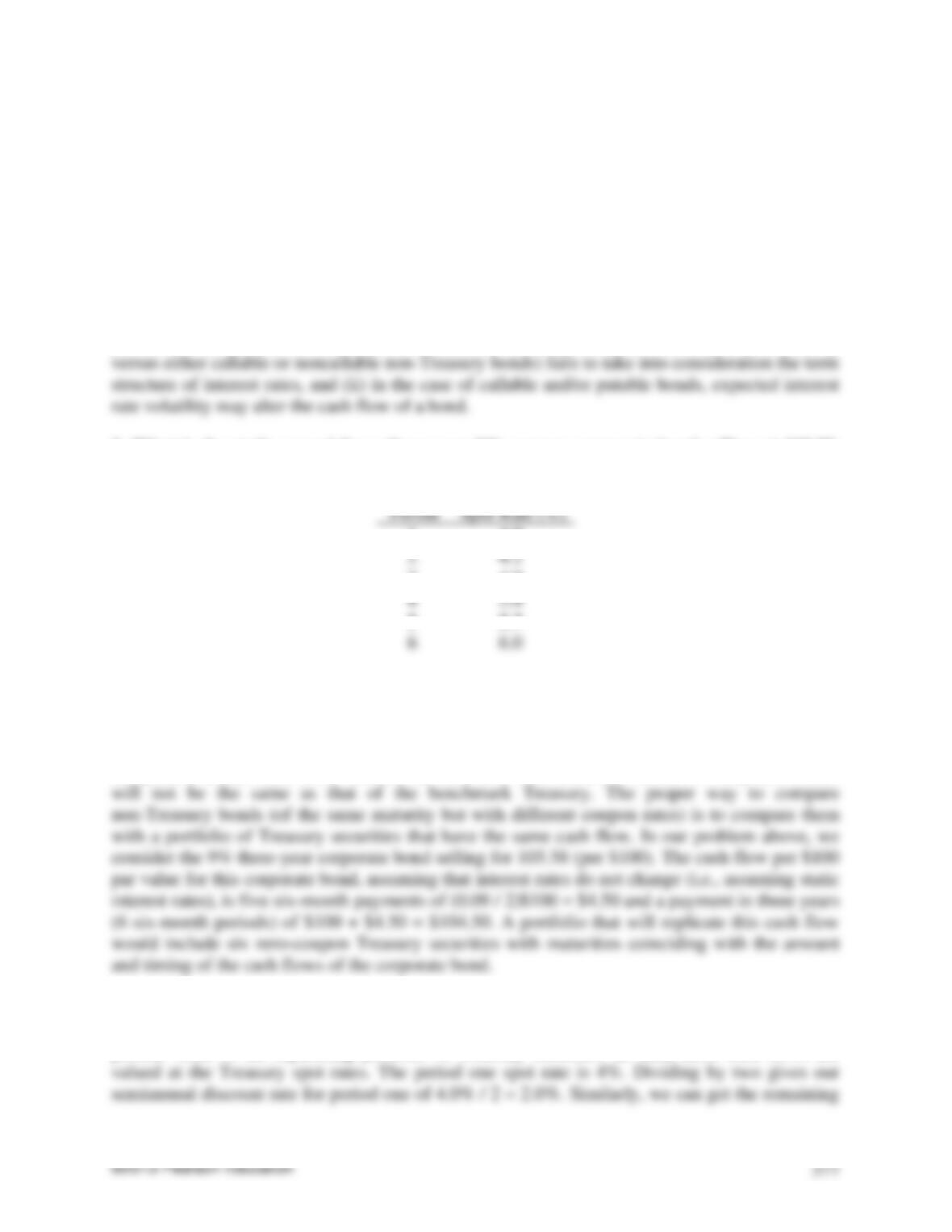
2. What is the static spread for a three-year 9% coupon corporate bond selling at 105.58,

given the following theoretical Treasury spot rate values equal to 50, 100, or 120 basis

points?

Period

Spot Rate (%)

1

4.0

2

4.2

3

4.9

4

5.4

5

5.7

6

6.0

In traditional yield spread analysis, an investor compares the yield to maturity of a bond with the

yield to maturity of a similar maturity on-the-run Treasury security. This means that the yield to

maturity of a three-year zero-coupon corporate bond and a 9% coupon three-year corporate

coupon bond would both be compared to a benchmark three-year Treasury security. Such a

comparison makes little sense because the cash flow characteristics of the two corporate bonds

The corporate bond’s value (105.58 quote per $100) is equal to the present value of all the cash

flows. The corporate bond’s value, assuming that the cash flows are riskless, will equal the

present value of the replicating portfolio of Treasury securities. In turn, these cash flows are

378

five semiannual discount rates for periods two through six which are 2.1%, 2.45%, 2.7%, 2.85%,

and 3.0%, respectively. Using our six semiannual discount rates, we get:

( ) ( ) ( ) ( ) ( )

2 3 4 5 6

$4.50 $4.50 $4.50 $4.50 $4.50 $100 $4.50

1.02 1.021 1.0245 1.027 1.0285 1.03

+

=$4.4118 + $4.3168 + $4.1848 + $4.0451 + $3.9101 + $84.5171 = $108.3857.

Thus, the price given the Treasury spot rates is $108.3857. However, the corporate bond’s price is

$105.58, which is less than the package of zero-coupon Treasury securities. This is because

investors require a yield premium for the risk associated with holding a corporate bond rather than

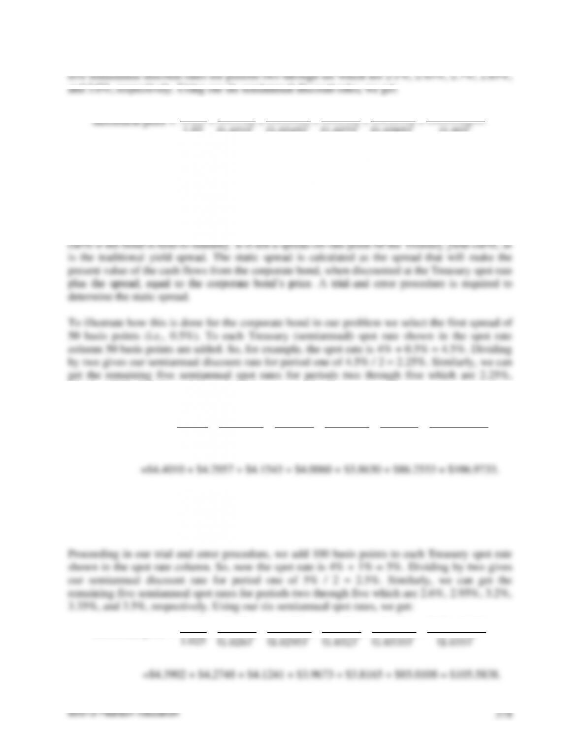
a riskless package of Treasury securities. The static spread, also referred to as the zero-volatility

spread, is a measure of the spread that the investor would realize over the entire Treasury spot rate

2.35%, 2.70%, 2.95%, 3.10%, and 3.25%, respectively. Using our six semiannual spot rates, we

get:

theoretical price =

( ) ( ) ( ) ( ) ( )

2 3 4 5 6

$4.50 $4.50 $4.50 $4.50 $4.50 $100 $4.50

1.0225 1.0235 1.027 1.0295 1.031 1.0325

+

+ + + + +

Thus, the spot rate plus 50 basis points renders a present value of $106.9733, which is greater

than the corporate bond’s price of $105.58. Thus, the static spread is not 50 basis points but must

be a higher spread. We will try 100 basis points.

theoretical price =

( ) ( ) ( ) ( ) ( )

2 3 4 5 6

$4.50 $4.50 $4.50 $4.50 $4.50 $100 $4.50

1.025 1.026 1.0295 1.032 1.0335 1.035

+

+ + + + +

Thus, the spot rate plus 100 basis points renders a present value of $105.5838, which rounded off

equals that corporate bond’s price of $105.58. Thus, the static spread appears to be 100 basis

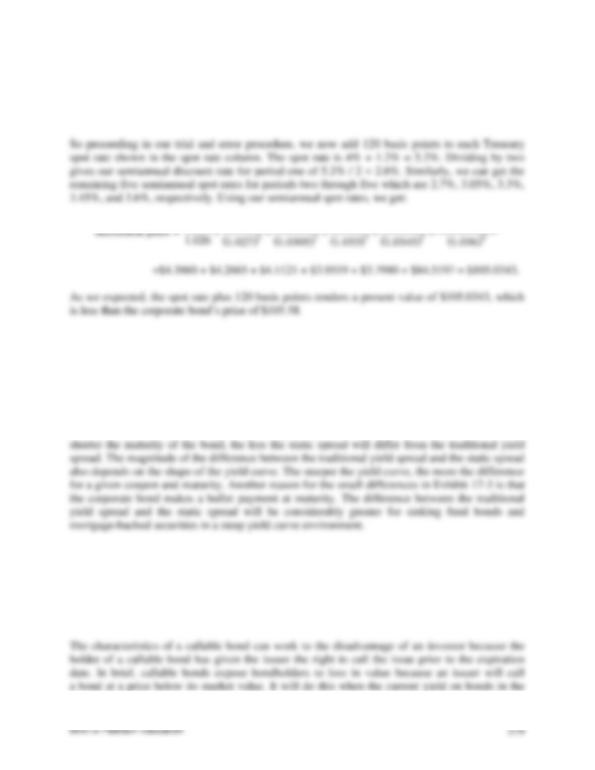
points. Although, we have our answer, we will go ahead and try 120 basis points given in our

problem.

$4.50 $4.50 $4.50 $4.50 $4.50 $100 $4.50

+

380

market is lower than the issue’s coupon rate. For example, if the coupon rate on a callable

corporate bond is 12% and prevailing market yields are 8%, the issuer may find it economical to

call the 12% issue and refund it with an 8% issue. From the investor’s perspective, the proceeds

received will have to be reinvested at a lower interest rate. This is called reinvestment risk.

Relatedly, the price appreciation potential for a callable bond in a declining interest-rate

environment is limited. This is because the market will increasingly expect the bond to be

redeemed at the call price as interest rates fall. This phenomenon for a callable bond is referred

to as price compression. Because of the disadvantages associated with callable bonds, these

instruments often feature a period of call protection, an initial period when bonds may not be

called. Also, the investor receives compensation in the form of a higher potential yield.

5. What is negative convexity?

6. Does a callable bond exhibit negative or positive convexity?

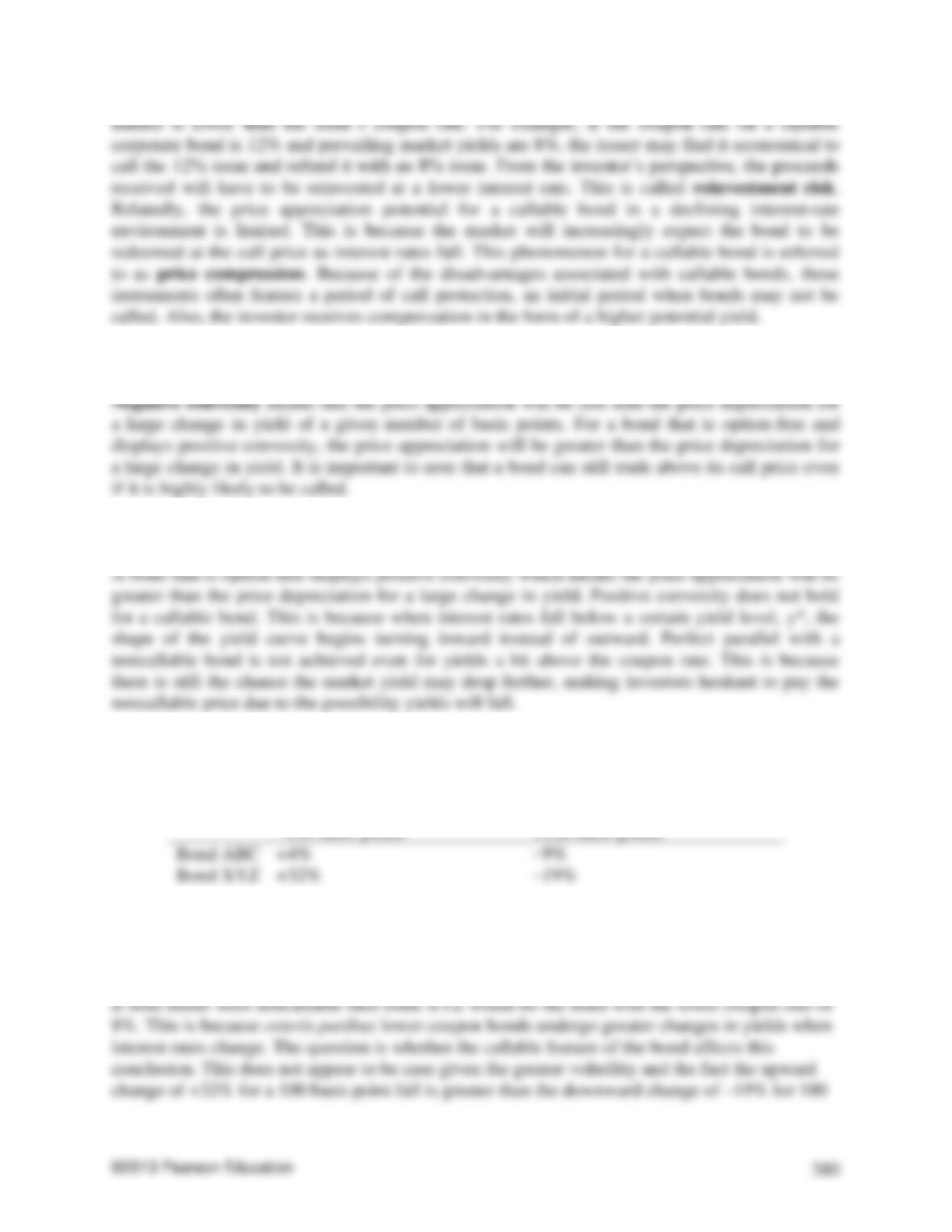
7. Suppose that you are given the following information about two callable bonds that can

be called immediately:

Estimated Percentage Change in Price if Interest Rates Change by:

–100 basis points

+100 basis points

Bond ABC

+4%

–9%

Bond XYZ

+32%

–19%

You are told that both of these bonds have the same maturity and that the coupon rate of

one bond is 8% and of the other is 14%. Suppose that the yield curve for both issuers is flat

at 9%. Based on this information, which bond is the lower coupon bond and which is the

higher coupon bond? Explain why.

381

basis points rise. Positive convexity means the bond will have greater price appreciation than

price depreciation for a large change in yield. This describes the situation for bond XYZ

indicating it is the bond with the lower coupon rate of 8%. This implies that bond ABC is the

bond with the higher coupon rate of 14%.

[Note. Bond XYZ exhibits positive convexity, and bond ABC exhibits negative convexity.

Assuming the same strike (call) price and the same current market yield, bond XYZ is less likely

to be called than is bond ABC. One might notice that comparing the percentage price change can

result in the same conclusion, but the reasoning is different.]

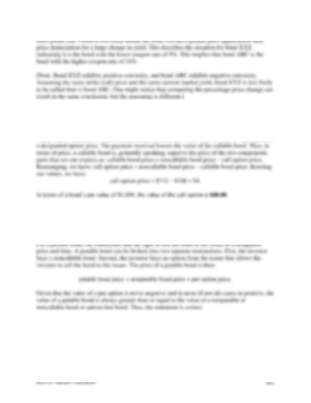
8. The theoretical value of a noncallable bond is $112; the theoretical value of a callable

bond is $108. Determine the theoretical value of the call option.

Effectively, the owner of a callable bond is entering into two separate transactions. First, the

owner buys a noncallable bond from the issuer. Second, the owner sells the issuer a call option at

9. Explain why you agree or disagree with the following statement: “The value of a putable

bond is never smaller than the value of an otherwise comparable option-free bond.”

As described below, one would agree with the statement.

10. Is it possible for an investor to pay more than the call price pay more than the call price

for a bond that is likely to be called?

It is possible for an investor to pay more than the call price, and it could be illustrated by the

following example.

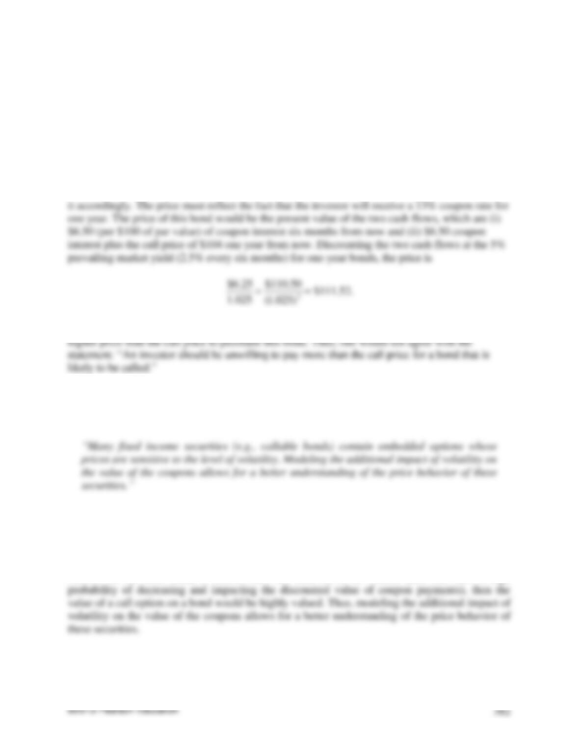
Consider a callable bond with a 10-year 13% coupon rate that is callable in one year at a call

price of 104. Suppose that the yield on 10-year bonds is 6% and that the yield on one-year bonds

is 5%. In a 6% interest rate environment for 10-year bonds, investors will expect that the issue

will be called in one year. Thus investors will treat this issue as if it is a one-year bond and price

2

)025.1(

025.1

The price is greater than the call price. Consequently, an investor would be willing to pay a

11. In Robert Litterman, Jose Scheinkman, and Laurence Weiss, “Volatility and the Yield

Curve,”Journal of Fixed Income, Premier Issue, 1991, p. 49, the following statement was

made:

Explain why.

The probability of a bond being called is a function of the volatility for of interest rates. If

expectations are that interest rates will not change (e.g., a flat yield curve) for a prolonged period

of time approaching the maturity of the bond, then the option to call a bond would not be highly

valued. On the other hand, if interest rates are believed to be volatile (and thus have a high