Chapter 16 – Managing Bond Portfolios
16-1
CHAPTER 16: MANAGING BOND PORTFOLIOS
PROBLEM SETS
1. While it is true that short-term rates are more volatile than long-term rates, the longer
2. Duration can be thought of as a weighted average of the ‘maturities’ of the cash flows
paid to holders of the perpetuity, where the weight for each cash flow is equal to the
3. The percentage change in the bond’s price is:
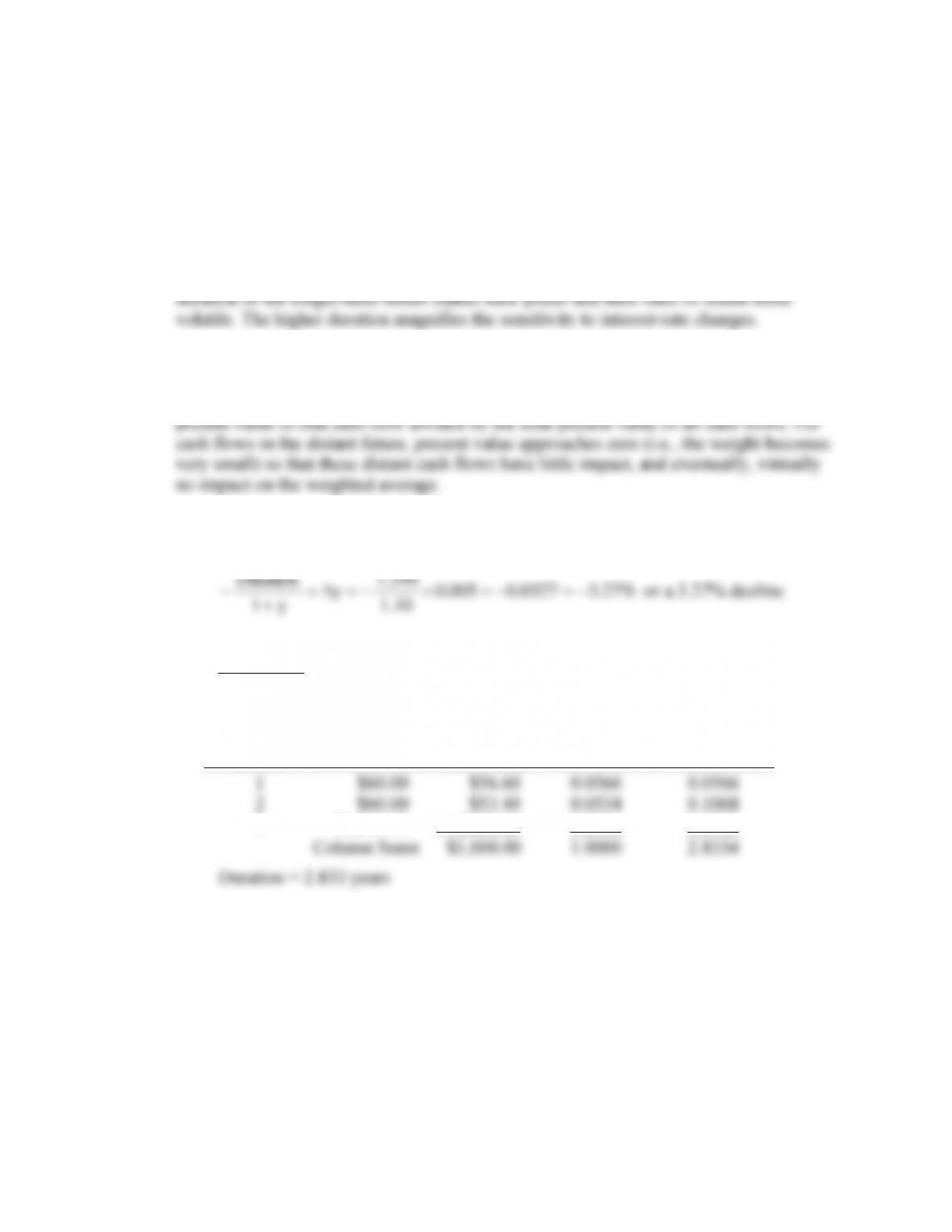
%27.30327.0005.0
10.1
194.7
y
y1
Duration −=−=−=
+
−
or a 3.27% decline
4. a. YTM = 6%
(1)
(2)
(3)
(4)
(5)
Time until
Payment
(years)
Cash Flow
PV of CF
(Discount
rate = 6%)
Weight
Column (1)
Column (4)
1
$60.00
$56.60
0.0566
0.0566
2
$60.00
$53.40
0.0534
0.1068
3
$1,060.00
$890.00
0.8900
2.6700
Column Sums
$1,000.00
1.0000
2.8334
Chapter 16 – Managing Bond Portfolios
16-2
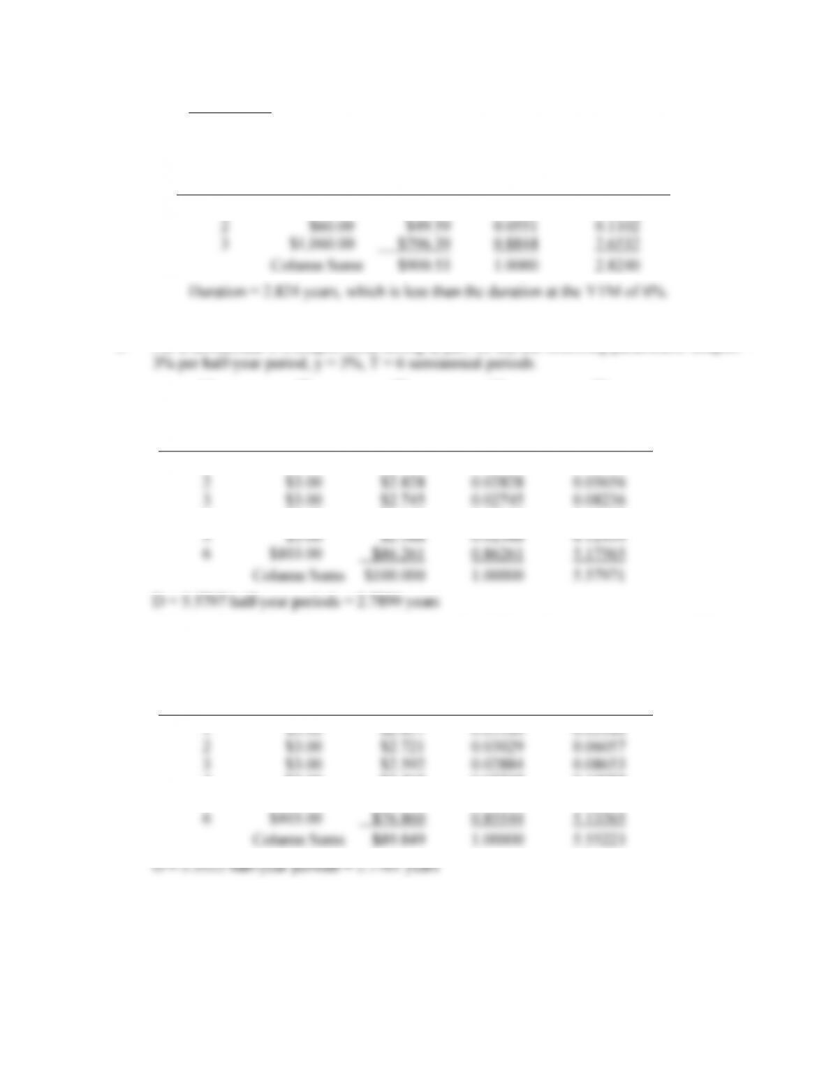
b. YTM = 10%
(1)
(2)
(3)
(4)
(5)
Time until
Payment
(years)
Cash Flow
PV of CF
(Discount
rate = 10%)
Weight
Column (1)
Column (4)
1
$60.00
$54.55
0.0606
0.0606
2
$60.00
$49.59
0.0551
0.1102
3
$1,060.00
$796.39
0.8844
2.6532
Column Sums
$900.53
1.0000
2.8240
5. For a semiannual 6% coupon bond selling at par, we use the following parameters: coupon =
(1)
(2)
(3)
(4)
(5)
Time until
Payment
(years)
Cash Flow
PV of CF
(Discount
rate = 3%)
Weight
Column (1)
Column (4)
1
$3.00
$2.913
0.02913
0.02913
2
$3.00
$2.828
0.02828
0.05656
3
$3.00
$2.745
0.02745
0.08236
4
$3.00
$2.665
0.02665
0.10662
5
$3.00
$2.588
0.02588
0.12939
6
$103.00
$86.261
0.86261
5.17565
Column Sums
$100.000
1.00000
5.57971
If the bond’s yield is 10%, use a semiannual yield of 5%, and semiannual coupon of 3%:
(1)
(2)
(3)
(4)
(5)
Time until
Payment
(years)
Cash Flow
PV of CF
(Discount
rate = 5%)
Weight
Column (1)
Column (4)
1
$3.00
$2.857
0.03180
0.03180
2
$3.00
$2.721
0.03029
0.06057
3
$3.00
$2.592
0.02884
0.08653
4
$3.00
$2.468
0.02747
0.10988
5
$3.00
$2.351
0.02616
0.13081
6
$103.00
$76.860
0.85544
5.13265
Column Sums
$89.849
1.00000
5.55223
Chapter 16 – Managing Bond Portfolios
6. a. Bond B has a higher yield to maturity than bond A since its coupon payments and
maturity are equal to those of A, while its price is lower. (Perhaps the yield is
b. Bond A has a lower yield and a lower coupon, both of which cause Bond A to
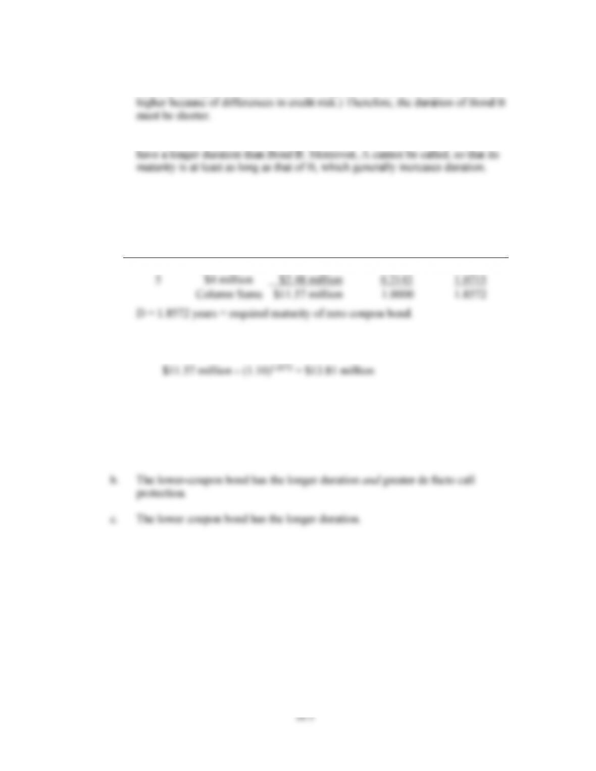
7. a.
(1)
(2)
(3)
(4)
(5)
Time until
Payment
(years)
Cash Flow
PV of CF
(Discount rate =
10%)
Weight
Column (1)
Column (4)
1
$10 million
$9.09 million
0.7857
0.7857
5
$4 million
$2.48 million
0.2143
1.0715
Column Sums
$11.57 million
1.0000
1.8572
b. The market value of the zero must be $11.57 million, the same as the market value
of the obligations. Therefore, the face value must be:
8. In each case, choose the longer-duration bond in order to benefit from a rate
decrease.
a. The Aaa-rated bond has the lower yield to maturity and therefore the longer
duration.
16-5
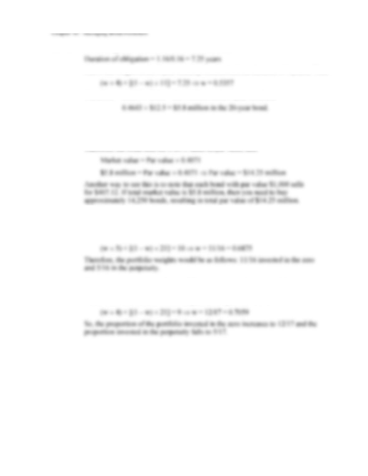
11. a. PV of obligation = $2 million/0.16 = $12.5 million
Call w the weight on the 5-year maturity bond (which has duration of 4 years). Then:
Therefore: 0.5357 $12.5 = $6.7 million in the 5-year bond and
b. The price of the 20-year bond is:
[$60 Annuity factor (16%, 20)] + [$1,000 PV factor (16%, 20)] = $407.12
Therefore, the bond sells for 0.4071 times its par value, and:
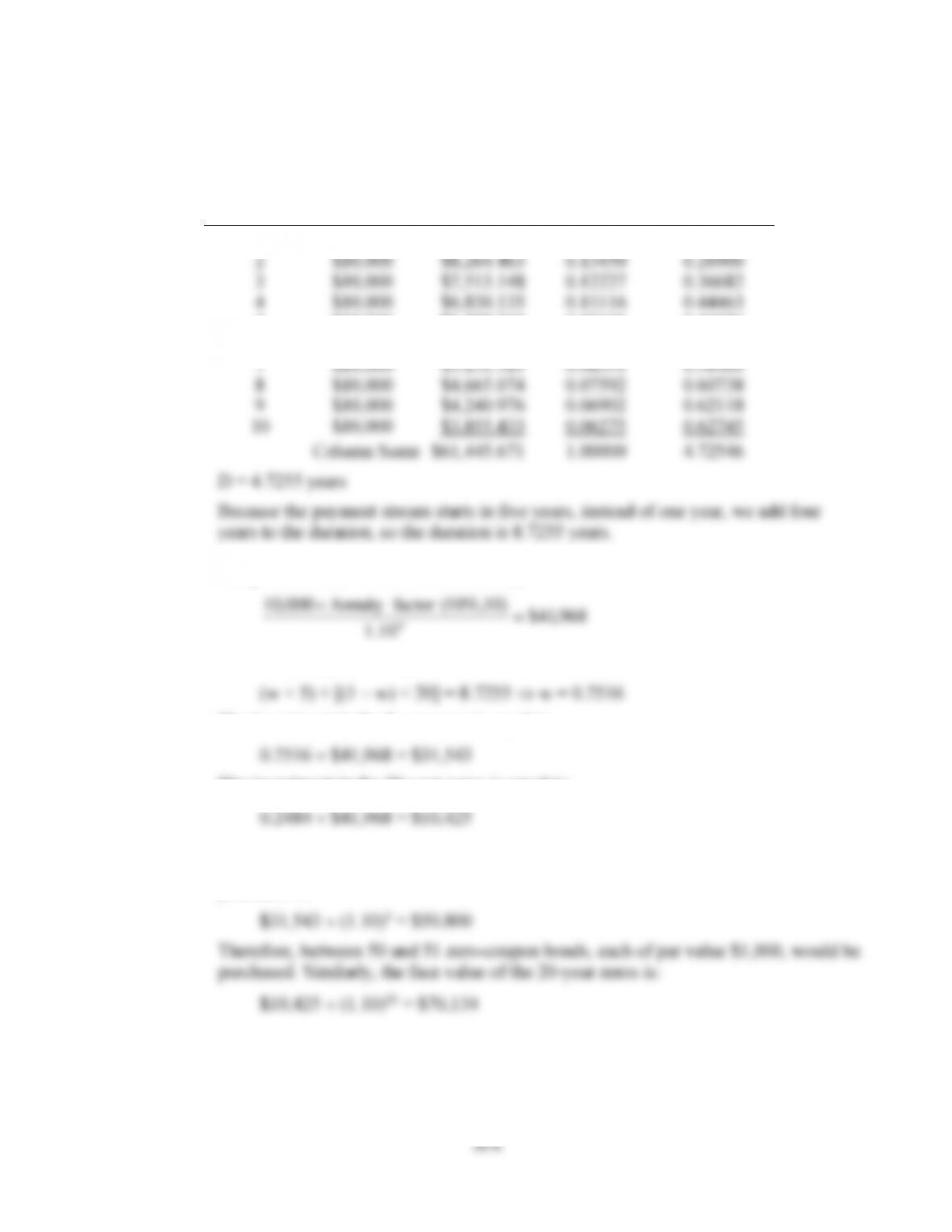
12. a. The duration of the perpetuity is: 1.05/0.05 = 21 years
Call w the weight of the zero-coupon bond. Then:
b. Next year, the zero-coupon bond will have a duration of 4 years and the perpetuity
will still have a 21-year duration. To obtain the target duration of nine years,
which is now the duration of the obligation, we again solve for w:
Chapter 16 – Managing Bond Portfolios
13. a. The duration of the annuity if it were to start in 1 year would be:
(1)
(2)
(3)
(4)
(5)
Time until
Payment
(years)
Cash Flow
PV of CF
(Discount
rate = 10%)
Weight
Column (1)
Column (4)
1
$10,000
$9,090.909
0.14795
0.14795
2
$10,000
$8,264.463
0.13450
0.26900
3
$10,000
$7,513.148
0.12227
0.36682
4
$10,000
$6,830.135
0.11116
0.44463
5
$10,000
$6,209.213
0.10105
0.50526
6
$10,000
$5,644.739
0.09187
0.55119
7
$10,000
$5,131.581
0.08351
0.58460
8
$10,000
$4,665.074
0.07592
0.60738
9
$10,000
$4,240.976
0.06902
0.62118
10
$10,000
$3,855.433
0.06275
0.62745
Column Sums
$61,445.671
1.00000
4.72546
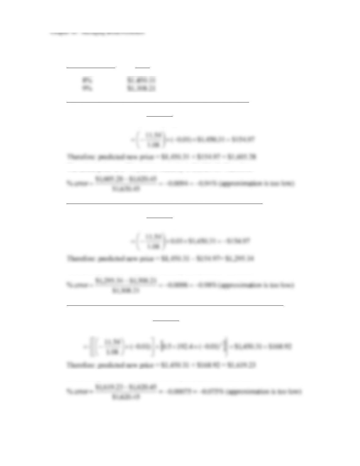
b. The present value of the deferred annuity is:
968,41$
10.1
)10%,10(factor Annuity 000,10
4=
Call w the weight of the portfolio invested in the 5-year zero. Then:
The investment in the 5-year zero is equal to:
The investment in the 20-year zeros is equal to:
These are the present or market values of each investment. The face values are
equal to the respective future values of the investments. The face value of the 5-
year zeros is:
16-7
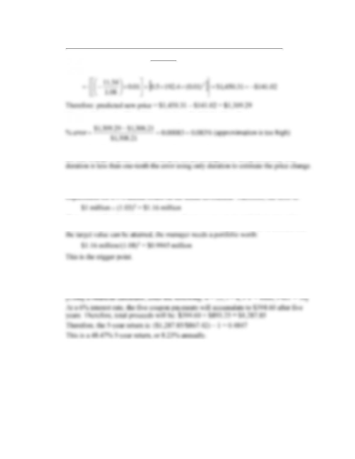
14. Using a financial calculator, we find that the actual price of the bond as a function of
yield to maturity is:
Yield to maturity Price
7% $1,620.45
Using the Duration Rule, assuming yield to maturity falls to 7%:
Predicted price change
0
Py
y1
Duration
+
−=
97.154$31.450,1$)01.0(
08.1
54.11 =−
−=
Therefore: predicted new price = $1,450.31 + $154.97 = $1,605.28
The actual price at a 7% yield to maturity is $1,620.45. Therefore:
45.620,1$
45.620,1$28.605,1$ −=−=
−
Using the Duration Rule, assuming yield to maturity increases to 9%:
Predicted price change
0
Py
y1
Duration
+
−=
97.154$31.450,1$01.0
08.1
54.11 −=
−=
Therefore: predicted new price = $1,450.31 – $154.97= $1,295.34
The actual price at a 9% yield to maturity is $1,308.21. Therefore:
21.308,1$
21.308,1$34.295,1$ −=−=
−
Using Duration-with-Convexity Rule, assuming yield to maturity falls to 7%
Predicted price change
0
2P)y(Convexity5.0y
y1
Duration
+
+
−=
92.168$31.450,1$)01.0(4.1925.0)01.0(
08.1
54.11 2=
−+
−
−=
Therefore: predicted new price = $1,450.31 + $168.92 = $1,619.23
The actual price at a 7% yield to maturity is $1,620.45. Therefore:
45.620,1$
45.620,1$23.619,1$ −=−=
−
Chapter 16 – Managing Bond Portfolios
16-8
Using Duration-with-Convexity Rule, assuming yield to maturity rises to 9%:
Predicted price change
0
2P)y(Convexity5.0y
y1
Duration
+
+
−=
02.141$31.450,1$)01.0(4.1925.001.0
08.1
54.11 2−=
+
−=
Therefore: predicted new price = $1,450.31 – $141.02 = $1,309.29
The actual price at a 9% yield to maturity is $1,308.21. Therefore:
21.308,1$
21.308,1$29.309,1$ ==
−
Conclusion: The duration-with-convexity rule provides more accurate approximations to
the true change in price. In this example, the percentage error using convexity with
15. The minimum terminal value that the manager is willing to accept is determined by the
Three years after the initial investment, only two years remain until the horizon date,
and the interest rate has risen to 8%. Therefore, at this time, in order to be assured that
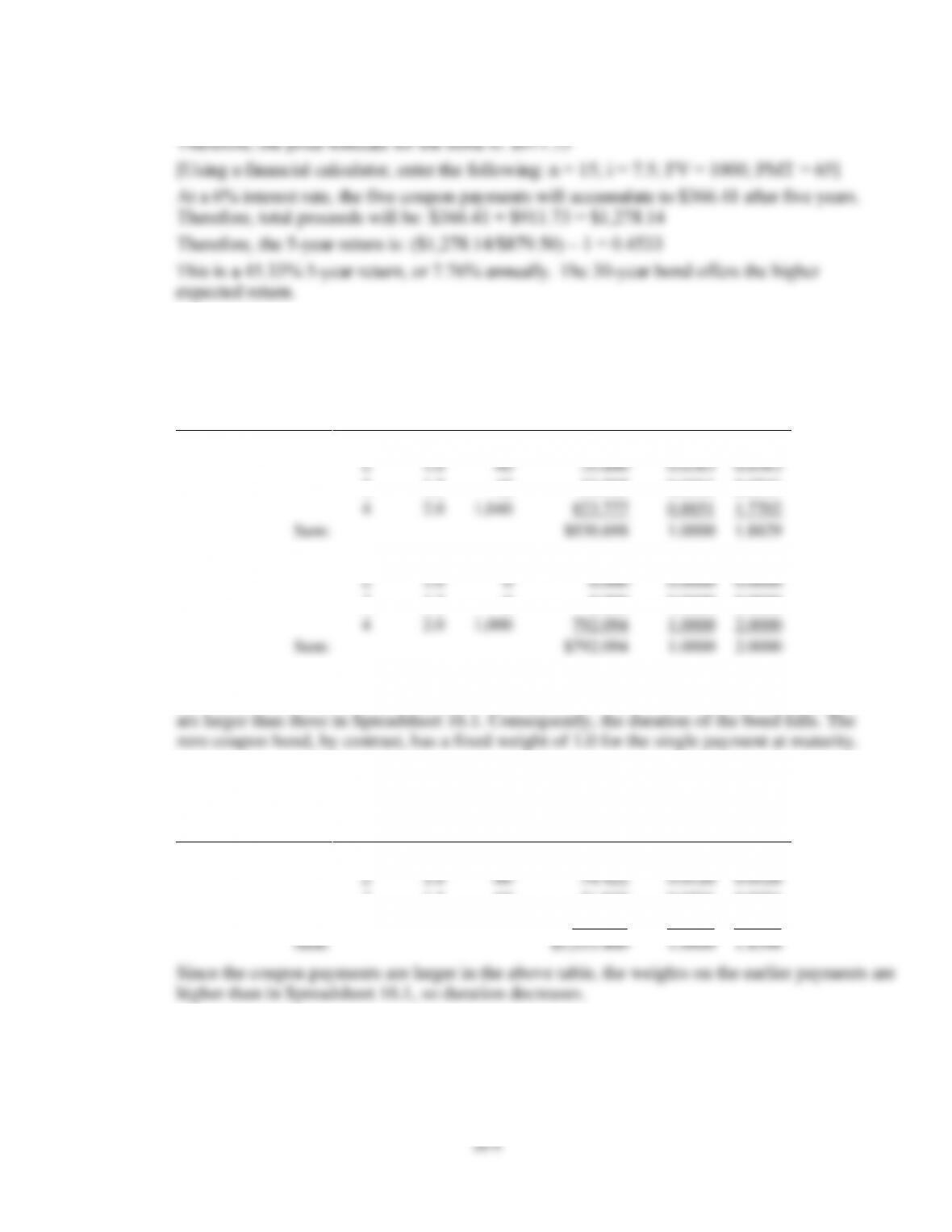
16. The maturity of the 30-year bond will fall to 25 years, and its yield is forecast to be 8%.
Therefore, the price forecast for the bond is: $893.25
Chapter 16 – Managing Bond Portfolios
The maturity of the 20-year bond will fall to 15 years, and its yield is forecast to be 7.5%.
17.
a.
Period
Time
until
Payment
(Years)
Cash
Flow
PV of CF
Discount rate =
6% per period
Weight
Years
Weight
A. 8% coupon bond
1
0.5
$40
$37.736
0.0405
0.0203
2
1.0
40
35.600
0.0383
0.0383
3
1.5
40
33.585
0.0361
0.0541
4
2.0
1,040
823.777
0.8851
1.7702
Sum:
$930.698
1.0000
1.8829
B. Zero-coupon
1
0.5
$0
$0.000
0.0000
0.0000
2
1.0
0
0.000
0.0000
0.0000
3
1.5
0
0.000
0.0000
0.0000
4
2.0
1,000
792.094
1.0000
2.0000
Sum:
$792.094
1.0000
2.0000
For the coupon bond, the weight on the last payment in the table above is less than it is in
Spreadsheet 16.1 because the discount rate is higher; the weights for the first three payments
b.
Period
Time
until
Payment
(Years)
Cash
Flow
PV of CF
Discount rate =
5% per period
Weight
Years
Weight
A. 8% coupon bond
1
0.5
$60
$57.143
0.0552
0.0276
2
1.0
60
54.422
0.0526
0.0526
3
1.5
60
51.830
0.0501
0.0751
4
2.0
1,060
872.065
0.8422
1.6844
Sum:
$1,035.460
1.0000
1.8396
16–10
18.
a.
Time
(t)
Cash
Flow
PV(CF)
t + t2
(t + t2) PV(CF)
Coupon =
$80
1
$80
$72.727
2
145.455
YTM =
0.10
2
80
66.116
6
396.694
Maturity =
5
3
80
60.105
12
721.262
Price =
$924.184
4
80
54.641
20
1,092.822
5
1,080
670.595
30
20,117.851
Price:
$924.184
Sum:
22,474.083
Convexity =
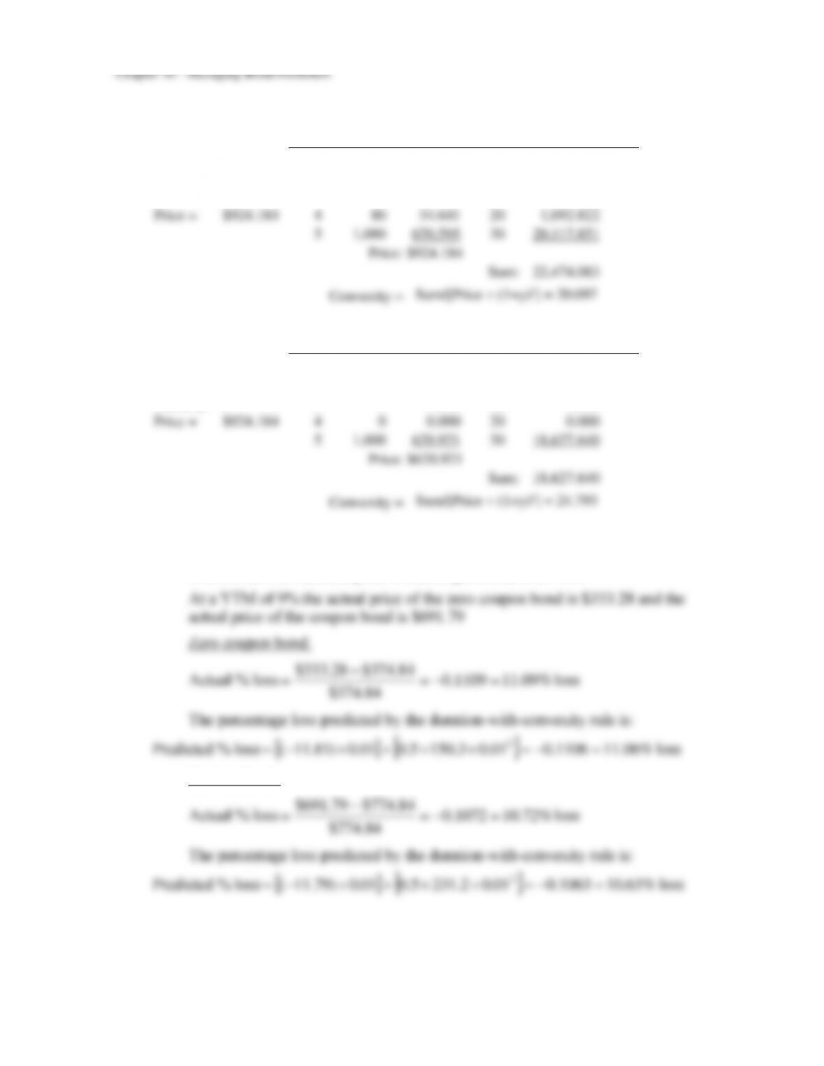
Sum/[Price (1+y)2] = 20.097
b.
Time
(t)
Cash
Flow
PV(CF)
t2 + t
(t2 + t) PV(CF)
Coupon =
$0
1
$0
$0.000
2
0.000
YTM =
0.10
2
0
0.000
6
0.000
Maturity =
5
3
0
0.000
12
0.000
Price =
$924.184
4
0
0.000
20
0.000
5
1,000
620.921
30
18,627.640
Price:
$620.921
Sum:
18,627.640
Convexity =
Sum/[Price (1+y)2] = 24.793
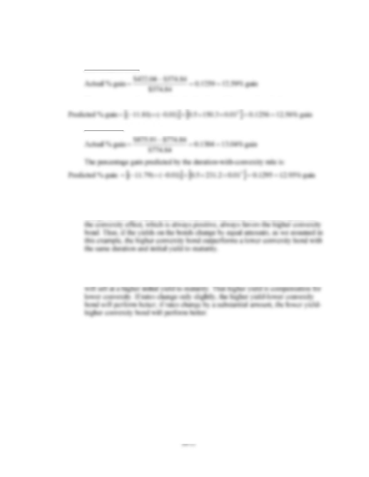
19. a. The price of the zero coupon bond ($1,000 face value) selling at a yield to maturity
of 8% is $374.84 and the price of the coupon bond is $774.84
Coupon bond:
84.774$79.691$ =−=
−
Chapter 16 – Managing Bond Portfolios
b. Now assume yield to maturity falls to 7%. The price of the zero increases to
$422.04, and the price of the coupon bond increases to $875.91
Zero coupon bond:
84.374$
84.374$04.422$==
−
The percentage gain predicted by the duration-with-convexity rule is:
Coupon bond
84.774$91.875$==
−
c. The 6% coupon bond, which has higher convexity, outperforms the zero regardless
of whether rates rise or fall. This can be seen to be a general property using the
duration-with-convexity formula: the duration effects on the two bonds due to any
change in rates are equal (since the respective durations are virtually equal), but
d. This situation cannot persist. No one would be willing to buy the lower convexity
bond if it always underperforms the other bond. The price of the lower convexity
bond will fall and its yield to maturity will rise. Thus, the lower convexity bond
16–12
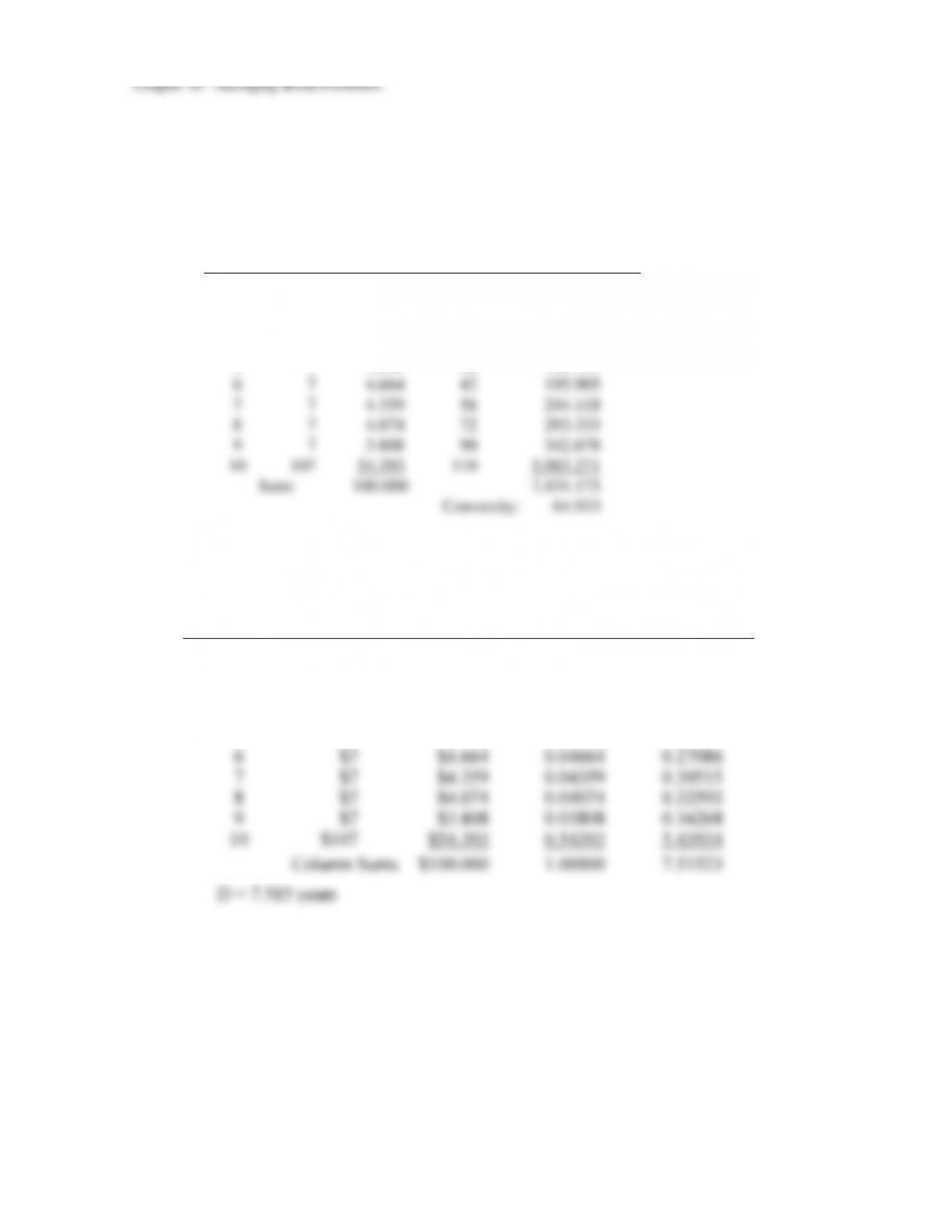
20. a. The following spreadsheet shows that the convexity of the bond is 64.933. The
present value of each cash flow is obtained by discounting at 7%. (Since the bond
has a 7% coupon and sells at par, its YTM is 7%.)
Convexity equals: the sum of the last column (7,434.175) divided by:
[P (1 + y)2] = 100 (1.07)2 = 114.49
Time
(t)
Cash flow
(CF)
PV(CF)
t2 + t
(t2 + t) × PV(CF)
1
7
6.542
2
13.084
2
7
6.114
6
36.684
3
7
5.714
12
68.569
4
7
5.340
20
106.805
5
7
4.991
30
149.727
6
7
4.664
42
195.905
7
7
4.359
56
244.118
8
7
4.074
72
293.333
9
7
3.808
90
342.678
10
107
54.393
110
5,983.271
Sum:
100.000
7,434.175
Convexity:
64.933
The duration of the bond is:
(1)
(2)
(3)
(4)
(5)
Time until
Payment
(years)
Cash Flow
PV of CF
(Discount
rate = 7%)
Weight
Column (1)
Column (4)
1
$7
$6.542
0.06542
0.06542
2
$7
$6.114
0.06114
0.12228
3
$7
$5.714
0.05714
0.17142
4
$7
$5.340
0.05340
0.21361
5
$7
$4.991
0.04991
0.24955
6
$7
$4.664
0.04664
0.27986
7
$7
$4.359
0.04359
0.30515
8
$7
$4.074
0.04074
0.32593
9
$7
$3.808
0.03808
0.34268
10
$107
$54.393
0.54393
5.43934
Column Sums
$100.000
1.00000
7.51523
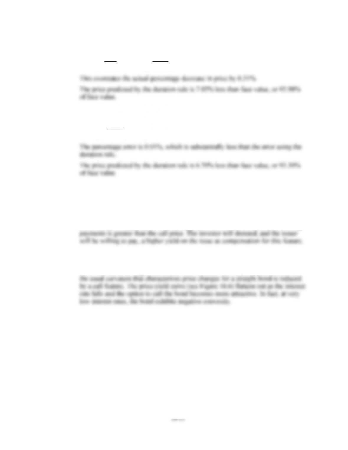
b. If the yield to maturity increases to 8%, the bond price will fall to 93.29% of par
value, a percentage decrease of 6.71%.
Chapter 16 – Managing Bond Portfolios
c. The duration rule predicts a percentage price change of:
%02.70702.001.0
07.1
515.7
01.0
07.1
D−=−=
−=
−
d. The duration-with-convexity rule predicts a percentage price change of:
%70.60670.001.0933.645.001.0
07.1
515.7 2−=−=+
−
CFA PROBLEMS
1. a. The call feature provides a valuable option to the issuer, since it can buy back the
bond at a specified call price even if the present value of the scheduled remaining
b. The call feature reduces both the duration (interest rate sensitivity) and the
convexity of the bond. If interest rates fall, the increase in the price of the callable
bond will not be as large as it would be if the bond were noncallable. Moreover,
16–14
2. a. Bond price decreases by $80.00, calculated as follows:
10 0.01 800 = 80.00
3. a. Modified duration
26.9
08.1
10
YTM1
durationMacaulay ==
+
=
years
b. For option-free coupon bonds, modified duration is a better measure of the bond’s
sensitivity to changes in interest rates. Maturity considers only the final cash flow,
while modified duration includes other factors, such as the size and timing of
c. i. Modified duration increases as the coupon decreases.
d. Convexity measures the curvature of the bond’s price-yield curve. Such curvature
means that the duration rule for bond price change (which is based only on the
2
P
4. a. (i) Current yield = Coupon/Price = $70/$960 = 0.0729 = 7.29%
Chapter 16 – Managing Bond Portfolios
16–15
(iii) Horizon yield or realized compound yield is 4.166% (semiannually), or
8.332% annual bond equivalent yield. To obtain this value, first find the future
value (FV) of reinvested coupons and principal. There will be six payments of $35
each, reinvested semiannually at 3% per period. On a financial calculator, enter:
b. Shortcomings of each measure:
(i) Current yield does not account for capital gains or losses on bonds bought at prices
other than par value. It also does not account for reinvestment income on coupon
payments.
(ii) Yield to maturity assumes the bond is held until maturity and that all coupon
income can be reinvested at a rate equal to the yield to maturity.
5. a. (i) The effective duration of the 4.75% Treasury security is:
2575.15
02.0
100/)372.86887.116(
r
P/P =
−
=
−
(ii) The duration of the portfolio is the weighted average of the durations of the
Chapter 16 – Managing Bond Portfolios
16–16
b. VanHusen’s remarks would be correct if there were a small, parallel shift in yields.
Duration is a first (linear) approximation only for small changes in yield. For
larger changes in yield, the convexity measure is needed in order to approximate
6. a. The Aa bond initially has a higher YTM (yield spread of 40 b.p. versus 31 b.p.),
but it is expected to have a widening spread relative to Treasuries. This will reduce
the rate of return. The Aaa spread is expected to be stable. Calculate comparative
returns as follows:
Incremental return over Treasuries =
b. Other variables to be considered:
• Potential changes in issue-specific credit quality. If the credit quality of the
bonds changes, spreads relative to Treasuries will also change.
• Changes in relative yield spreads for a given bond rating. If quality spreads
7. a. % price change = (−Effective duration) Change in YTM (%)
Chapter 16 – Managing Bond Portfolios
b. Since we are asked to calculate horizon return over a period of only one coupon
period, there is no reinvestment income.
Horizon return = Coupon payment +Year-end price − Initial Price
Initial price
50.017,1$50.055,1$25.31$==
−+
Chapter 16 – Managing Bond Portfolios
16–18
b. A change in yield spreads across sectors would call for an intermarket spread
swap, in which the manager buys bonds in the sector for which yields are expected
c. A belief that the yield spread on a particular instrument will change calls for a
substitution swap in which that security is sold if its yield is expected to rise
10. a. The advantages of a bond indexing strategy are:
• Historically, the majority of active managers underperform benchmark indexes in
most periods; indexing reduces the possibility of underperformance at a given
level of risk.
• Indexed portfolios do not depend on advisor expectations and so have less risk of
underperforming the market.
• Management advisory fees for indexed portfolios are dramatically less than fees
for actively managed portfolios. Fees charged by active managers generally
• Plan sponsors have greater control over indexed portfolios because individual
managers do not have as much freedom to vary from the parameters of the
The disadvantages of a bond indexing strategy are:
• Indexed portfolio returns may match the bond index, but do not necessarily
reflect optimal performance. In some time periods, many active managers may
Chapter 16 – Managing Bond Portfolios
16–19
b. The stratified sampling, or cellular, method divides the index into cells, with each
cell representing a different characteristic of the index. Common cells used in the
cellular method combine (but are not limited to) duration, coupon, maturity,
c. Tracking error is defined as the discrepancy between the performance of an
indexed portfolio and the benchmark index. When the amount invested is
relatively small and the number of cells to be replicated is large, a significant
11. a. For an option-free bond, the effective duration and modified duration are
approximately the same. Using the data provided, the duration is calculated as
follows:
100.7
002.0
100/)29.9971.100(
r
P/P =
−
=
−
b. The total percentage price change for the bond is estimated as follows:
c. The assistant’s argument is incorrect. Because modified convexity does not recognize
the fact that cash flows for bonds with an embedded option can change as yields
change, modified convexity remains positive as yields move below the callable bond’s
Chapter 16 – Managing Bond Portfolios
12. ∆P/P = −D* ∆y
For Strategy I:
13. a. i. Strong economic recovery with rising inflation expectations. Interest rates and
bond yields will most likely rise, and the prices of both bonds will fall. The
probability that the callable bond will be called would decrease, and the callable
bond will behave more like the non-callable bond. (Note that they have similar
b. Projected price change = (modified duration) (change in YTM)
c. For Bond A, the callable bond, bond life and therefore bond cash flows are uncertain.
If one ignores the call feature and analyzes the bond on a “to maturity” basis, all
calculations for yield and duration are distorted. Durations are too long and yields are
too high. On the other hand, if one treats the premium bond selling above the call price