CHAPTER 16
INTEREST-RATE MODELS
CHAPTER SUMMARY
In implementing bond portfolio strategies there are two important activities that a manager will
undertake. First, a manager will want to determine whether the bonds that are purchase and sale
candidates are fairly priced. Second, a manager will want to assess the performance of a portfolio
over realistic future interest-rate scenarios. For both of these activities, the manager will have to
MATHEMATICAL DESCRIPTION OF ONE-FACTOR INTEREST-RATE MODELS
Interest-rate models must incorporate statistical properties of interest-rate movements. These
properties are (1) drift, (2) volatility, and (3) mean reversion. The commonly used mathematical
tool for describing the movement of interest rates that can incorporate these properties is
stochastic differential equations (SDEs).
The most common interest-rate model used to describe the behavior of interest rates assumes that
short-term interest rates follow some statistical process and that other interest rates in the term
structure are related to short-term rates. The short-term interest rate (i.e., short rate) is the only
one that is assumed to drive the rates of all other maturities. Hence, these models are referred to
In all of these models because time is a continuous variable, the letter d is used to denote the
“change in” some variable. Specifically, in the models we let
r = the short rate and therefore dr denotes the change in the short rate
t = time and thus dt denotes the change in time (or the length of the time interval)
z = a random term and dz denotes a random process
A Basic Continuous-Time Stochastic Process
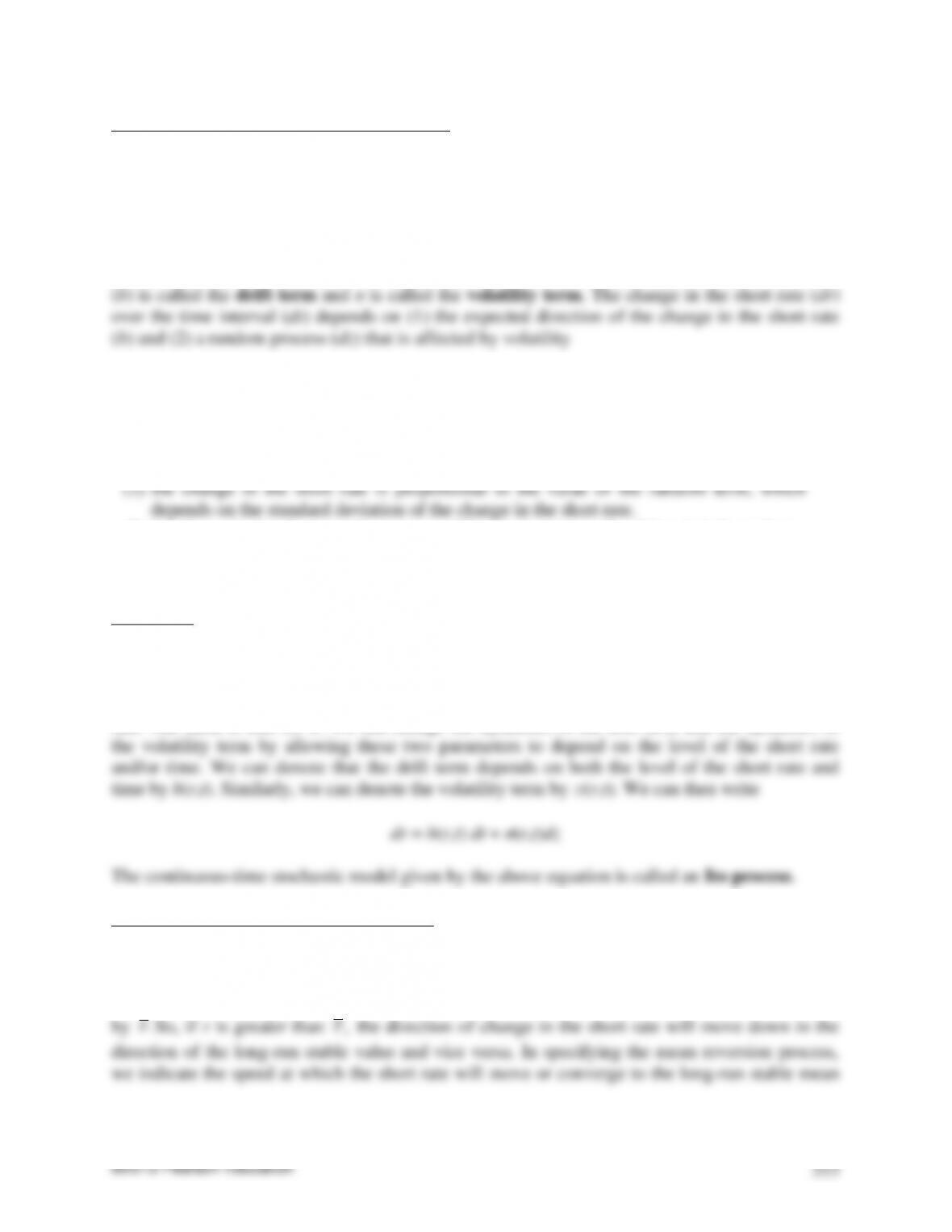
We begin with a basic continuous-time stochastic process for describing the dynamics of the
short rate given by: dr = bdt + σdz
where dr, dt, and dz were defined above, σ = standard deviation of the changes in the short rate,
and b = expected direction of rate change. The expected direction of the change in the short rate
The random nature of the change in the short rate comes from the random process dz. The
assumptions are that
(1) the random term z follows a normal distribution with a mean of zero and a standard
deviation of one (i.e., is a standardized normal distribution).
(3) the change in the short rate for any two different short intervals of time is independent.
Based on the assumptions above, important properties can be shown.
Itô Process
In the above equation, neither the drift term nor the standard deviation of the change in the short
rate depends on the level of the short rate and time. There are economic reasons that might
suggest that the expected direction of the rate change will depend on the level of the current short
rate. The same is true for σ. We can change the dynamics of the drift term and the dynamics of
Specifying the Dynamics of the Drift Term
In specifying the dynamics of the drift term, one can specify that the drift term depends on the
level of the short rate by assuming it follows a mean reversion process. By mean reversion it is
meant that some long-run stable mean value for the short rate is assumed. We denote this value
value. This parameter is called the speed of adjustment and we will denote it by α. The mean
reversion process that specifies the dynamics of the drift term is:
Specifying the Dynamics of the Volatility Term
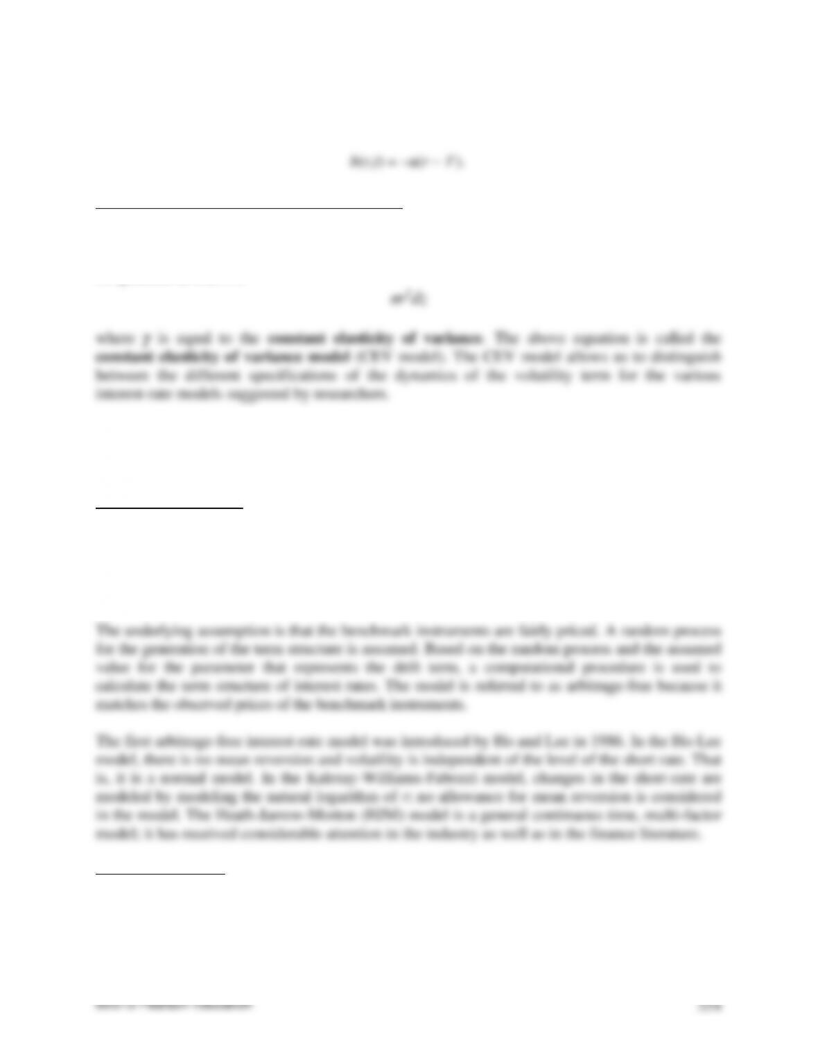
There have been several formulations of the dynamics of the volatility term. If volatility is not
assumed to depend on time, then σ(r,t) = σ(r). In general, the dynamics of the volatility term can
be specified as follows:
ARBITRAGE-FREE VERSUS EQUILIBRIUM MODELS
Interest-rate models fall into two general categories: arbitrage models and equilibrium models.
Arbitrage-Free Models
In arbitrage-free models, also referred to as no-arbitrage models, the analysis begins with the
observed market price of a set of financial instruments. The financial instruments can include
cash market instruments and interest-rate derivatives, and they are referred to as the benchmark
instruments or reference set.
Equilibrium Models
A fair characterization of arbitrage-free models is that they allow one to interpolate the term
structure of interest rates from a set of observed market prices at one point in time assuming that
one can rely on the market prices used. Equilibrium models, however, are models that seek to
describe the dynamics of the term structure using fundamental economic variables that are
assumed to affect the interest-rate process. In the modeling process, restrictions are imposed
allowing for the derivation of closed-form solutions for equilibrium prices of bonds and interest
rate derivatives. In these models (1) a functional form of the interest-rate volatility is assumed
and (2) how the drift moves up and down over time is assumed.
EMPIRICAL EVIDENCE ON INTEREST-RATE CHANGES
In any review of interest-rate models, one encounters the following issues: (1) the choice
between normal models (i.e., volatility is independent of the level of interest rates) and logarithm
models; and, (2) if interest rates are highly unlikely to be negative, then interest-rate models that
allow for negative rates may be less suitable as a description of the interest-rate process.
Volatility of Rates and the Level of Interest Rates
The dependence of volatility on the level of interest rates has been examined by several
researchers. The earlier research focused on short-term rates and gave inconclusive findings.
Oren Cheyette found that for different periods there are different degrees of dependence of
volatility on the level of interest rates. However, when interest rates were below 10%, the
Negative Interest Rates
While our focus is on nominal interest rates, we know that real interest rates have been found to
be negative on only rare occasions. The reason is that if the nominal rate is negative, investors
will simply hold cash. It is fair to say that while negative interest rates are not impossible, they
SELECTING AN INTEREST-RATE MODEL
The ease of application is a critical issue in selecting an interest-rate model. For consistency in
valuation, a portfolio manager would want a model that can be used to value all financial
instruments that are included in a portfolio. In practice, writing efficient algorithms to value all
financial instruments that may be included in a portfolio for some interest-rate models that have
been proposed in the literature is “difficult or impossible.”
ESTIMATING INTEREST-RATE VOLATILITY USING HISTORICAL DATA
One of the inputs into an interest-rate model is interest-rate volatility. Where does a practitioner
obtain this value in order to implement an interest-rate model? Market participants estimate yield
volatility in one of two ways. The first way is by estimating historical interest volatility. This
method uses historical interest rates to calculate the standard deviation of interest-rate changes
and for obvious reasons is referred to as historical volatility. The second method is more
KEY POINTS
• An interest-rate model is a probabilistic description of how interest rates can change over
time. A stochastic differential equation is the most commonly used mathematical tool for
describing interest-rate movements that incorporate statistical properties of interest-rate
movements (drift, volatility, and mean reversion).
• In a one-factor model, the SDE expresses the interest rate movement in terms of the change in
the short rate over the time interval based on two components: (1) the expected direction of
the change in the short rate (the drift term), and (2) a random process (the volatility term).
• Interest-rate models fall into two general categories: arbitrage-free models and equilibrium
models.
• For arbitrage-free models, the analysis begins with the observed market price of benchmark
instruments that are assumed to be fairly priced, and using those prices one derives a term
structure that is consistent with observed market prices for the benchmark instruments. The
model is referred to as arbitrage-free because it matches the observed prices of the benchmark
instruments.
• Interest-rate volatility can be estimated using historical volatility or implied volatility.
• Historical volatility is calculated from observed rates over some period of time. When
calculating historical volatility using daily observations, differences in annualized volatility
occur for a given set of observations because of the different assumptions that can be made
about the number of trading days in a year. Implied volatility is obtained using an option
pricing model and observed prices for option-type derivative instruments.
ANSWERS TO QUESTIONS FOR CHAPTER 16
(Questions are in bold print followed by answers.)
1. What is meant by an interest-rate model?
By an interest rate model, we mean a model that incorporates statistical properties of interest-rate
movements. These properties are (1) drift, (2) volatility, and (3) mean reversion. The commonly
used mathematical tool for describing the movement of interest rates that can incorporate these
properties is stochastic differential equations (SDEs).
2. Answer the below questions.
(a) Explain the drift property found in an interest-rate model.
The drift term refers to that variable in an interest rate model that captures the expected
direction of the change in the interest rate (e.g., a short-term nominal rate referred to as the short
rate). The symbol b is used in interest rate models to represent the drift. Various assumptions
(b) Explain the volatility property found in an interest-rate model.
The volatility term refers to that variability of the interest rate or the short rate. The symbol σ is
used in interest rate models to represent the volatility and is simply the standard deviation of the
changes in the short rate. Like the drift term, assumptions are made such as its dependency on
the level of the short rate. There have been several formulations of the dynamics of the volatility
term. If volatility is assumed to depend on time, then we express volatility asσ(r,t) where r is the
(c) Explain the mean reversion property found in an interest-rate model.
By the mean reversion property, it is meant that some long-run stable mean value for the short
rate is assumed. This long-run value can be denoted by
r
. So, if the short-rate (r) is greater than
r
, the direction of change in the short rate will move down in the direction of the long-run
stable value and vice versa. However, in specifying the mean reversion process, it is necessary to
r
3. What is the commonly used mathematical tool for describing the movement of interest
rates that can incorporate the properties of an interest-rate model?
The commonly used mathematical tool for describing the movement of interest rates (that can
incorporate the properties of drift, volatility and mean reversion) is stochastic differential
equations (SDEs). A rigorous treatment of interest-rate modeling requires an understanding of
this specialized topic in mathematics. It is also worth noting that SDEs are used in the pricing of
options. More details are given below.
The most common interest-rate model used to describe the behavior of interest rates assumes that
short-term interest rates follow some statistical process and that other interest rates in the term
structure are related to short-term rates. The short-term interest rate (i.e., short rate) is the only
While the value of the short rate at some future time is uncertain, the pattern by which it changes
over time can be assumed. In statistical terminology, this pattern or behavior is called a
stochastic process. Thus, describing the dynamics of the short rate means specifying the
stochastic process that describes the movement of the short rate. It is assumed that the short rate
is a continuous random variable and therefore the stochastic process used is a continuous-time
4. Answer the below questions.
(a) Why is the most common interest-rate model used to describe the behavior of interest
rates a one-factor model?
In practice, one-factor models are used because of the difficulty of applying even a two-factor
model. In addition, there is empirical evidence that supports one-factor models. Thus, due to the
greater simplicity and applicability of one-factor models, they are preferred over two-factor
models.
(b) What is the one-factor in a one-factor interest-rate model?
The one-factor in a one-factor interest-rate model is short-term interest rates where it is assumed
short rates follow some statistical process with other interest rates in the term structure related to
the short rate. Thus, the short rate is the only factor that is assumed to drive the rates of all other
maturities.
5. Answer the below questions.
(a) What is meant by a normal model of interest rates?
The classification of a model as normal is based on the assumed dynamics of the random
component of the stochastic differential equation (SDE). Normal models assume that interest rate
volatility is independent of the level of rates and therefore admits the possibility of negative
interest rates. More details are given below.
(b) What is meant by a lognormal model of interest rates?
Like a normal model, the classification of a model as lognormal is based on the assumed
dynamics of the random component of the SDE. However, unlike normal models, lognormal
models assume that interest-rate volatility is proportional to the level of rates, and therefore
negative interest rates are not possible. An example of a lognormal model is the
Kalotay-Williams-Fabozzi (KWF) model where changes in the short-rate are modeled by
modeling the natural logarithm of r; no allowance for mean reversion is considered in the model.
©2013 Pearson Education
361
rates than the lognormal model. Moreover, empirical tests suggest that the impact of negative
interest rates on pricing is minimal, and therefore one should not be overly concerned that
a normal model admits the possibility of negative interest rates.
6. Answer the below questions.
a. Explain the treatment of the dynamics of the volatility term for the Vasicek interest rate
model.
Let us begin by noting that there have been several formulations of the dynamics of the volatility
term. If volatility is not assumed to depend on time, then σ(r,t) = σ(r). In general, the dynamics
of the volatility term can be specified as follows:
σrγdz
b. Explain the treatment of the dynamics of the volatility term for the Dothan interest rate
model.
For the Dothan interest rate model, we look at the case for γ = 1. Substituting this value for γ into
σrγdz, we get the following model identified by Dothan who first proposed it:
γ = 1: σ(r,t) = σ r (Dothan specification of CEV model).
c. Explain the treatment of the dynamics of the volatility term for the Cox-Ingersoll-Ross
interest rate model.
For the Cox-Ingersoll-Ross specification interest rate model, we look at the case for γ = 1/2.
Substituting this value for γ into σrγdz, we get the following model identified by Cox-Ingersoll-Ross
who first proposed it:
©2013 Pearson Education
362
γ = 1/2: σ(r,t) = σ
r
(Cox-Ingersoll-Ross specification).
The Cox-Ingersoll-Ross (CIR) specification, referred to as the square-root model, makes the
volatility proportional to the square rate of the short rate. Negative interest rates are not possible
in this square-root model.
One can combine the dynamics of the drift term and volatility term to create the following
commonly used interest rate model:
dr =
( )
αα− − +r r dt rdz
.
This model specifies a mean reversion process for the drift term and the square root model for
volatility and is referred to as the mean-reverting square-root model.
While there have been many developments in equilibrium models, the best known models are the
Vasicek and CIR models. To apply these models, estimates of the parameters of the assumed
interest-rate process are needed, including the parameters of the volatility function for interest
rates. These estimated parameters are typically obtained using econometric techniques that rely
on historical yield curves without regard to how the final model matches any market prices.
7. What is an arbitrage-free interest-rate model?
An arbitrage-free interest-rate model is a model that allows one to interpolate the term
structure of interest rates from a set of observed market prices at one point in time assuming that
one can rely on the market prices used. Thus, in arbitrage-free models, also referred to as
no-arbitrage models, the analysis begins with the observed market price of a set of financial
instruments. The financial instruments can include cash market instruments and interest-rate
8. Answer the below questions.
(a) What are the general characteristics of the Ho-Lee arbitrage-free interest-rate model?
The first arbitrage-free interest-rate model was introduced by Ho and Lee in 1986. In the Ho-Lee
model, there is no mean reversion and volatility is independent of the level of the short rate. That
is, it is a normal model [i.e., constant elasticity of variance (γ) = 0].
(b) How does the Ho-Lee arbitrage-free interest-rate model differ from the Hull-White
arbitrage-free interest-rate model?
9. What is an equilibrium interest-rate model?
An equilibrium interest-rate model is a model that seeks to describe the dynamics of the term
structure using fundamental economic variables that are assumed to affect the interest-rate
process. In the modeling process, restrictions are imposed allowing for the derivation of
closed-form solutions for equilibrium prices of bonds and interest rate derivatives. In these
models (1) a functional form of the interest-rate volatility is assumed and (2) how the drift moves
up and down over time is assumed. More details are given below.
10. Indicate whether you agree or disagree with the following statement: “In practice,
equilibrium models are typically used rather than arbitrage-free models”.
One would disagree about the statement. In practice, arbitrage-free models are typically used
because they are easier to implement than equilibrium models. To illustrate, there are two
concerns with implementing and using equilibrium models. First, many economic theories start
11. Answer the below questions.
(a) What is the empirical evidence on the relationship between volatility and the level of
interest rates?
Empirical evidence reviewed regarding the relationship between interest-rate volatility and the
level of rates suggests that the relationship is weak at interest rate levels below 10%. However,
for rates exceeding 10%, there tends to be a positive relationship. More details are given below.
To answer this question, we need to examine from an historical perspective the issue as to
whether interest rate volatility is affected by the level of interest rates or independent of the level
of interest rates. If it is affected, one might suspect a higher the level of interest rates will lead to
greater volatility in the interest rates. That is, there will be a positive correlation between the
level of interest rates and interest-rate volatility. If the two are independent, a low correlation
would exist.
(b) Explain whether the historical evidence supports the use of a normal model or a lognormal
model.
The support for a normal model or a lognormal model depends on the current level of interest
rates as described below.
Empirical evidence reviewed regarding the relationship between interest-rate volatility and the
level of rates suggests that the relationship is weak at interest rate levels below 10%. However,
for rates exceeding 10%, there tends to be a positive relationship. This evidence suggests that in
rate environments below 10%, a normal model would be more descriptive of the behavior of
©2013 Pearson Education
365
interest rates than the lognormal model. Moreover, empirical tests suggest that the impact of
negative interest rates on pricing is minimal, and therefore one should not be overly concerned
that a normal model admits the possibility of negative interest rates.
12. Comment on the following statement: “For an interest-rate model to be useful, the drift
term has to be a constant regardless it is a positive, zero or negative number.
13. Answer the below questions.
(a) What is meant by historical volatility?
By historical volatility is meant the degree of change in interest rates over some past time period.
More details are given below.
Market participants estimate yield volatility in one of two methods: historical volatility or
implied volatility. The historical interest volatility method uses historical interest rates to
calculate the standard deviation of interest-rate changes. The text uses to explain how to
The weekly measures must be annualized. The formula for annualizing a weekly standard
deviation is: weekly standard deviation ×
52
. Annualizing the two weekly volatility measures,
we have: absolute rate change = 2.32 ×
52
= 18.86 basis points and logarithm percent change =
1.33 ×
52
= 9.62%. If we use monthly data to compute the standard deviation, the following
(b) What is meant by implied volatility?
Market participants estimate yield volatility in one of two methods: historical volatility or
implied volatility. The implied volatility method is more complicated than the historical method
as it involves using models for valuing option-type derivative instruments to obtain an estimate
of what the market expects interest-rate volatility is. In any option pricing model, the only input
©2013 Pearson Education
366
that is not observed in the model is interest-rate volatility. In practice, one assumes that the
observed price for an option-type derivative is priced according to some option pricing model.
The calculation then involves determining what interest-rate volatility will make the market price
of the option-type derivative equal to the value generated by the option pricing model. Since the
expected interest-rate volatility obtained is being “backed out” of the model, it is referred to as
implied volatility.
14. Suppose that the following weekly interest-rate volatility estimates are computed as:
absolute rate change = 4.75 basis points
percentage rate change = 1.12%.
Answer the below questions.
(a) What is the annualized volatility for the absolute rate change?
(b) What is the annualized volatility for the percentage rate change?
15. Give an example to explain that one can combine the dynamics of the drift term and
volatility term to create an interest rate model.
In specifying the dynamics of the drift term, one can specify that the drift term depends on the
level of the short rate by assuming it follows a mean-reversion process. There have been
several formulations of the dynamics of the volatility term. In general, the dynamics of the
volatility term can be specified as follows:
dzr