
Chapter 13 – Empirical Evidence on Security Returns
13-1
CHAPTER 13: EMPIRICAL EVIDENCE ON SECURITY RETURNS
PROBLEM SETS
1. Even if the single-factor CCAPM (with a consumption-tracking portfolio used as the
index) performs better than the CAPM, it is still quite possible that the consumption
2. Wealth and consumption should be positively correlated and, therefore, market volatility
and consumption volatility should also be positively correlated. Periods of high market
volatility might coincide with periods of high consumption volatility. The
‘conventional’ CAPM focuses on the covariance of security returns with returns for the
market portfolio (which in turn tracks aggregate wealth) while the consumption-based

Chapter 13 – Empirical Evidence on Security Returns
13-2
Note: For the following problems, the focus is on the estimation procedure. To keep
3. Using the regression feature of Excel with the data presented in the text, the first-pass
(SCL) estimation results are:
Stock:
A
B
C
D
E
F
G
H
I
R Square
0.06
0.06
0.06
0.37
0.17
0.59
0.06
0.67
0.70
Observations
12
12
12
12
12
12
12
12
12
Alpha
9.00
-0.63
-0.64
-5.05
0.73
-4.53
5.94
-2.41
5.92
Beta
-0.47
0.59
0.42
1.38
0.90
1.78
0.66
1.91
2.08
t-Alpha
0.73
-0.04
-0.06
-0.41
0.05
-0.45
0.33
-0.27
0.64
t-Beta
-0.81
0.78
0.78
2.42
1.42
3.83
0.78
4.51
4.81
4. The hypotheses for the second-pass regression for the SML are:
5. The second-pass data from first-pass (SCL) estimates are:
Average
Excess
Return
Beta
A
5.18
-0.47
B
4.19
0.59
C
2.75
0.42
D
6.15
1.38
E
8.05
0.90
F
9.90
1.78
G
11.32
0.66
H
13.11
1.91
I
22.83
2.08
M
8.12

Chapter 13 – Empirical Evidence on Security Returns
13-3
The second-pass regression yields:
Regression Statistics
Multiple R
0.7074
R Square
0.5004
Adjusted R Square
0.4291
Standard Error
4.6234
Observations
9
Coefficients
Standard
Error
t Statistic
for
=0
t Statistic
for
=8.12
Intercept
3.92
2.54
1.54
Slope
5.21
1.97
2.65
-1.48
6. As we saw in the chapter, the intercept is too high (3.92% per year instead of 0) and the
slope is too flat (5.21% instead of a predicted value equal to the sample-average risk
7. Arranging the securities in three portfolios based on betas from the SCL estimates, the
first pass input data are:
Year
ABC
DEG
FHI
1
15.05
25.86
56.69
2
-16.76
-29.74
-50.85
3
19.67
-5.68
8.98
4
-15.83
-2.58
35.41
5
47.18
37.70
-3.25
6
-2.26
53.86
75.44
7
-18.67
15.32
12.50
8
-6.35
36.33
32.12
9
7.85
14.08
50.42
10
21.41
12.66
52.14
11
-2.53
-50.71
-66.12
12
-0.30
-4.99
-20.10
Average
4.04
8.51
15.28
Std. Dev.
19.30
29.47
43.96

Chapter 13 – Empirical Evidence on Security Returns
The first-pass (SCL) estimates are:
ABC
DEG
FHI
R Square
0.04
0.48
0.82
Observations
12
12
12
Alpha
2.58
0.54
-0.34
Beta
0.18
0.98
1.92
t-Alpha
0.42
0.08
-0.06
t-Beta
0.62
3.02
6.83
Grouping into portfolios has improved the SCL estimates as is evident from the higher
R-square for Portfolio DEG and Portfolio FHI. This means that the beta (slope) is
measured with greater precision, reducing the error-in-measurement problem at the
expense of leaving fewer observations for the second pass.
The inputs for the second pass regression are:
Average
Excess
Return
Beta
ABC
4.04
0.18
DEH
8.51
0.98
FGI
15.28
1.92
M
8.12
The second-pass estimates are:
Regression Statistics
Multiple R
0.9975
R Square
0.9949
Adjusted R
Square
0.9899
Standard Error
0.5693
Observations
3
Coefficients
Standard
Error
t Statistic
for
=0
t Statistic
for
=8.12
Intercept
2.62
0.58
4.55
Slope
6.47
0.46
14.03
-3.58
Despite the decease in the intercept and the increase in slope, the intercept is now
significantly positive, and the slope is significantly less than the hypothesized value by
more than three times the standard error.
13-5
8. Roll’s critique suggests that the problem begins with the market index, which is not the
9.
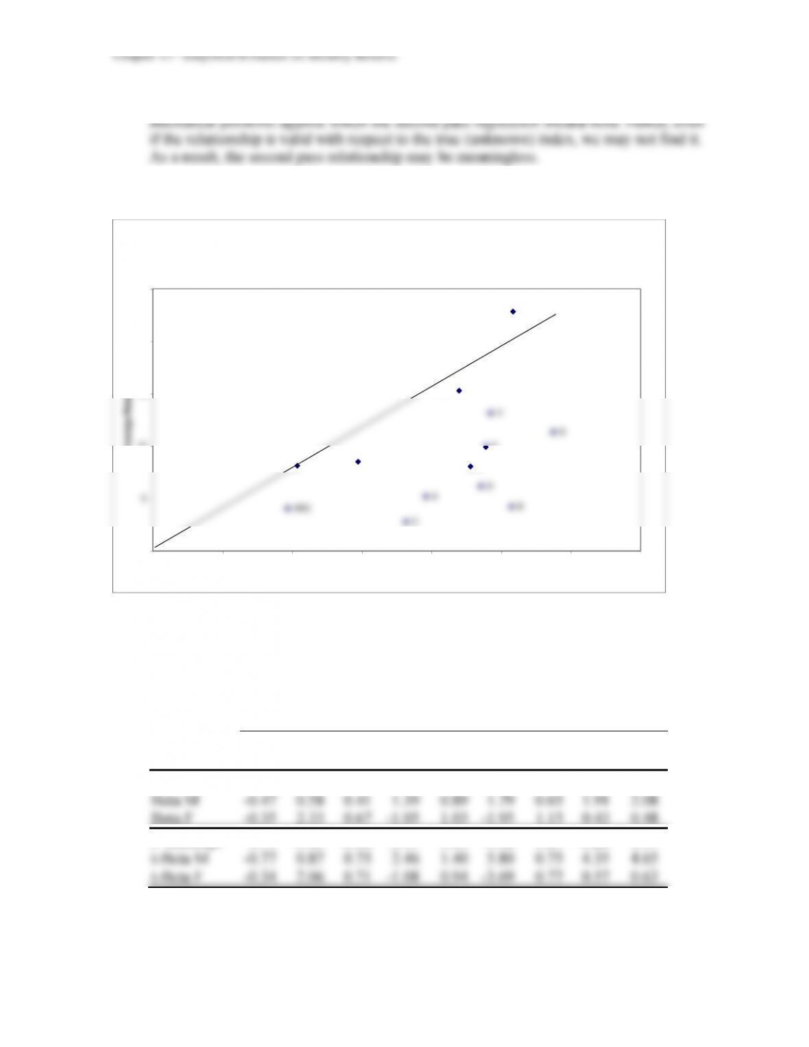
Except for Stock I, which realized an extremely positive surprise, the CML shows that
the index dominates all other securities, and the three portfolios dominate all individual
stocks. The power of diversification is evident despite the very small sample size.
10. The first-pass (SCL) regression results are summarized below:
A
B
C
D
E
F
G
H
I
R-Square
0.07
0.36
0.11
0.44
0.24
0.84
0.12
0.68
0.71
Observations
12
12
12
12
12
12
12
12
12
Intercept
9.19
-1.89
-1.00
-4.48
0.17
-3.47
5.32
-2.64
5.66
Beta M
-0.47
0.58
0.41
1.39
0.89
1.79
0.65
1.91
2.08
Beta F
-0.35
2.33
0.67
-1.05
1.03
-1.95
1.15
0.43
0.48
t- Intercept
0.71
-0.13
-0.08
-0.37
0.01
-0.52
0.29
-0.28
0.59
t-Beta M
-0.77
0.87
0.75
2.46
1.40
5.80
0.75
4.35
4.65
t-Beta F
-0.34
2.06
0.71
-1.08
0.94
-3.69
0.77
0.57
0.63
CAPITAL MARKET LINE FROM SAMPLE DATA
ABC
Market
DEG
C
B
A
D
E
F
G
H
FHI
I
0
5
10
15
20
25
010 20 30 40 50 60 70
Standard Deviation
Average Return
CML
Chapter 13 – Empirical Evidence on Security Returns
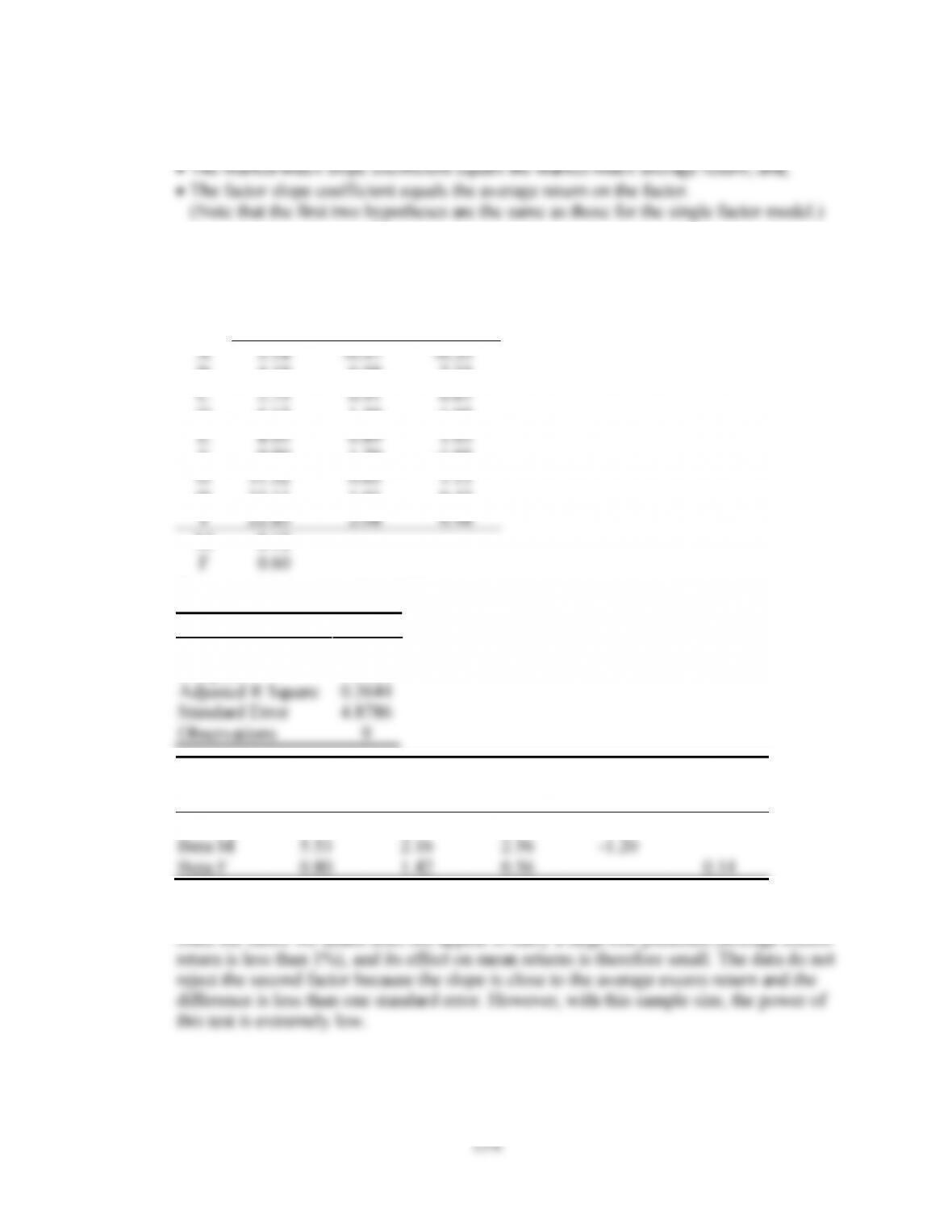
11. The hypotheses for the second-pass regression for the two-factor SML are:
• The intercept is zero;
12. The inputs for the second pass regression are:
Average
Excess
Return
Beta M
Beta F
A
5.18
-0.47
-0.35
B
4.19
0.58
2.33
C
2.75
0.41
0.67
D
6.15
1.39
-1.05
E
8.05
0.89
1.03
F
9.90
1.79
-1.95
G
11.32
0.65
1.15
H
13.11
1.91
0.43
I
22.83
2.08
0.48
M
8.12
F
0.60
The second-pass regression yields:
Regression Statistics
Multiple R
0.7234
R Square
0.5233
Adjusted R Square
0.3644
Standard Error
4.8786
Observations
9
Coefficients
Standard
Error
t Statistic
for
=0
t Statistic
for
=8.12
t Statistic
for
=0.6
Intercept
3.35
2.88
1.16
Beta M
5.53
2.16
2.56
-1.20
Beta F
0.80
1.42
0.56
0.14
These results are slightly better than those for the single factor test; that is, the intercept
is smaller and the slope on M is slightly greater. We cannot expect a great improvement
since the factor we added does not appear to carry a large risk premium (average excess

13-7
13. When we use the actual factor, we implicitly assume that investors can perfectly
replicate it, that is, they can invest in a portfolio that is perfectly correlated with the
factor. When this is not possible, one cannot expect the CAPM equation (the second
pass regression) to hold. Investors can use a replicating portfolio (a proxy for the factor)
that maximizes the correlation with the factor. The CAPM equation is then expected to
equal the factor mean of 0.60%. The resultant weights for the proxy and period returns
are:
Proxy Portfolio for Factor F (PF)
Weights on
Universe
Stocks
Year
PF Holding
Period
Returns
A
-0.14
1
-33.51
B
1.00
2
62.78
C
0.95
3
9.87
D
-0.35
4
-153.56
E
0.16
5
200.76
F
-1.00
6
-36.62
G
0.13
7
-74.34
H
0.19
8
-10.84
I
0.06
9
28.11
10
59.51
11
-59.15
12
14.22
Average
0.60
This proxy (PF) has an R-square with the actual factor of 0.80.
We next perform the first pass regressions for the two factor model using PF instead of
P:
A
B
C
D
E
F
G
H
I
R-square
0.08
0.55
0.20
0.43
0.33
0.88
0.16
0.71
0.72
Observations
12
12
12
12
12
12
12
12
12
Intercept
9.28
-2.53
-1.35
-4.45
-0.23
-3.20
4.99
-2.92
5.54
Beta M
-0.50
0.80
0.49
1.32
1.00
1.64
0.76
1.97
2.12
Beta PF
-0.06
0.42
0.16
-0.13
0.21
-0.29
0.21
0.11
0.08
t- Intercept
0.72
-0.21
-0.12
-0.36
-0.02
-0.55
0.27
-0.33
0.58
t-Beta M
-0.83
1.43
0.94
2.29
1.66
6.00
0.90
4.67
4.77
t-Beta PF
-0.44
3.16
1.25
-0.97
1.47
-4.52
1.03
1.13
0.78
Note that the betas of the nine stocks on M and the proxy (PF) are different from those
in the first pass when we use the actual proxy.

Chapter 13 – Empirical Evidence on Security Returns
13-8
The first-pass regression for the two-factor model with the proxy yields:
Average
Excess
Return
Beta M
Beta PF
A
5.18
-0.50
-0.06
B
4.19
0.80
0.42
C
2.75
0.49
0.16
D
6.15
1.32
-0.13
E
8.05
1.00
0.21
F
9.90
1.64
-0.29
G
11.32
0.76
0.21
H
13.11
1.97
0.11
I
22.83
2.12
0.08
M
8.12
PF
0.6
The second-pass regression yields:
Regression Statistics
Multiple R
0.71
R Square
0.51
Adjusted R Square
0.35
Standard Error
4.95
Observations
9
Coefficients
Standard
Error
t Statistic
for
=0
t Statistic
for
=8.12
t Statistic
for
=0.6
Intercept
3.50
2.99
1.17
Beta M
5.39
2.18
2.48
-1.25
Beta PF
0.26
8.36
0.03
-0.04
We can see that the results are similar to, but slightly inferior to, those with the actual
factor, since the intercept is larger and the slope coefficient smaller. Note also that we

Chapter 13 – Empirical Evidence on Security Returns
13-9
14. We assume that the value of your labor is incorporated in the calculation of the rate of
return for your business. It would likely make sense to commission a valuation of your
business at least once each year. The resultant sequence of figures for percentage change
in the value of the business (including net cash withdrawals from the business in the
calculations) will allow you to derive a reasonable estimate of the correlation between
the rate of return for your business and returns for other assets. You would then search
for industries having the lowest correlations with your portfolio, and identify exchange
CFA PROBLEMS
1. (i) Betas are estimated with respect to market indexes that are proxies for the true
market portfolio, which is inherently unobservable.
2. a. The basic procedure in portfolio evaluation is to compare the returns on a managed
portfolio to the return expected on an unmanaged portfolio having the same risk,
using the SML. That is, expected return is calculated from:
b. The benchmark error might occur when the unmanaged portfolio used in the
evaluation process is not “optimized.” That is, market indices, such as the S&P
500, chosen as benchmarks are not on the manager’s ex ante mean/variance
efficient frontier.

Chapter 13 – Empirical Evidence on Security Returns
c. Your graph should show an efficient frontier obtained from actual returns, and a
different one that represents (unobserved) ex-ante expectations. The CML and
d. The answer to this question depends on one’s prior beliefs. Given a consistent
track record, an agnostic observer might conclude that the data support the claim
e. The question is really whether the CAPM is at all testable. The problem is that
even a slight inefficiency in the benchmark portfolio may completely invalidate
any test of the expected return-beta relationship. It appears from Roll’s argument
3. The effect of an incorrectly specified market proxy is that the beta of Black’s portfolio is
likely to be underestimated (i.e., too low) relative to the beta calculated based on the
“true” market portfolio. This is because the Dow Jones Industrial Average (DJIA), and
other market proxies, are likely to have less diversification and therefore a higher
variance of returns than the “true” market portfolio as specified by the capital asset
2Proxy Market
Portfolio
An incorrectly specified market proxy is likely to produce a slope for the security
market line (i.e., the market risk premium) that is underestimated relative to the “true”
market portfolio. This results from the fact that the “true” market portfolio is likely to be