Chapter 10 – Arbitrage Pricing Theory and Multifactor Models of Risk and Return
CHAPTER 10: ARBITRAGE PRICING THEORY
AND MULTIFACTOR MODELS OF RISK AND RETURN
PROBLEM SETS
1. The revised estimate of the expected rate of return on the stock would be the old
2. The APT factors must correlate with major sources of uncertainty, i.e., sources of
uncertainty that are of concern to many investors. Researchers should investigate factors
3. Any pattern of returns can be “explained” if we are free to choose an indefinitely large
4. Equation 10.9 applies here:
E(rp) = rf + P1 [E(r1 ) − rf ] + P2 [E(r2) – rf ]
We need to find the risk premium (RP) for each of the two factors:
10-2
5. The expected return for Portfolio F equals the risk-free rate since its beta equals 0.
For Portfolio A, the ratio of risk premium to beta is: (12 − 6)/1.2 = 5
For Portfolio E, the ratio is lower at: (8 – 6)/0.6 = 3.33
This implies that an arbitrage opportunity exists. For instance, you can create a Portfolio
6. Substituting the portfolio returns and betas in the expected return-beta relationship, we
obtain two equations with two unknowns, the risk-free rate (rf ) and the factor risk
premium (RP):
12 = rf + (1.2 RP)
7. a. Shorting an equally-weighted portfolio of the ten negative-alpha stocks and
investing the proceeds in an equally-weighted portfolio of the ten positive-alpha
stocks eliminates the market exposure and creates a zero-investment portfolio.
Denoting the systematic market factor as RM , the expected dollar return is (noting
that the expectation of non-systematic risk, e, is zero):
$1,000,000 [0.02 + (1.0 RM )] − $1,000,000 [(–0.02) + (1.0 RM )]
Chapter 10 – Arbitrage Pricing Theory and Multifactor Models of Risk and Return
For n = 20 stocks (i.e., long 10 stocks and short 10 stocks) the investor will have a
$100,000 position (either long or short) in each stock. Net market exposure is zero,
but firm-specific risk has not been fully diversified. The variance of dollar returns
from the positions in the 20 stocks is:
b. If n = 50 stocks (25 stocks long and 25 stocks short), the investor will have a
$40,000 position in each stock, and the variance of dollar returns is:
50 [(40,000 0.30)2 ] = 7,200,000,000
The standard deviation of dollar returns is $84,853.
8. a.
)e(
22
M
22 +=
88125)208.0( 2222
A=+=
50010)200.1( 2222
B=+=
97620)202.1( 2222
C=+=
b. If there are an infinite number of assets with identical characteristics, then a well-
diversified portfolio of each type will have only systematic risk since the non-
c. There is no arbitrage opportunity because the well-diversified portfolios all plot on
10-4
9. a. A long position in a portfolio (P) comprised of Portfolios A and B will offer an
expected return-beta tradeoff lying on a straight line between points A and B.
Therefore, we can choose weights such that P = C but with expected return
b. The argument in part (a) leads to the proposition that the coefficient of 2 must be
b. Surprises in the macroeconomic factors will result in surprises in the return of the
stock:
Unexpected return from macro factors =
11. The APT required (i.e., equilibrium) rate of return on the stock based on rf and the
factor betas is:
12. The first two factors seem promising with respect to the likely impact on the firm’s cost of
capital. Both are macro factors that would elicit hedging demands across broad sectors of
investors. The third factor, while important to Pork Products, is a poor choice for a
Chapter 10 – Arbitrage Pricing Theory and Multifactor Models of Risk and Return
10-5
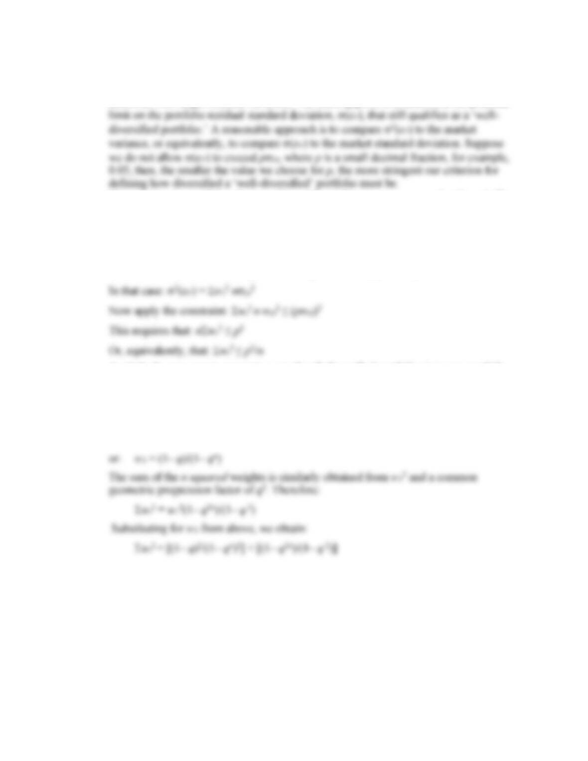
13. The maximum residual variance is tied to the number of securities (n) in the portfolio
because, as we increase the number of securities, we are more likely to encounter
securities with larger residual variances. The starting point is to determine the practical
Now construct a portfolio of n securities with weights w1, w2,…,wn, so that wi =1. The
portfolio residual variance is: 2(eP) = w122(ei)
To meet our practical definition of sufficiently diversified, we require this residual
variance to be less than (pM)2. A sure and simple way to proceed is to assume the
worst, that is, assume that the residual variance of each security is the highest possible
value allowed under the assumptions of the problem: 2(ei) = n2M
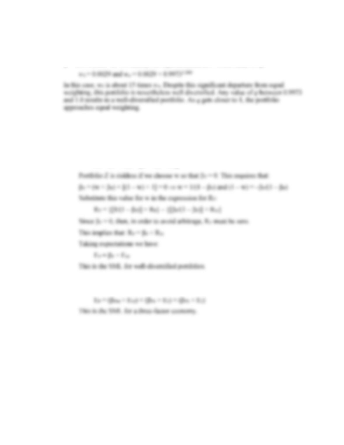
A relatively easy way to generate a set of well-diversified portfolios is to use portfolio
weights that follow a geometric progression, since the computations then become relatively
straightforward. Choose w1 and a common factor q for the geometric progression such that
q < 1. Therefore, the weight on each stock is a fraction q of the weight on the previous
stock in the series. Then the sum of n terms is:
wi = w1(1– qn)/(1– q) = 1
Chapter 10 – Arbitrage Pricing Theory and Multifactor Models of Risk and Return
10-6
For sufficient diversification, we choose q so that: wi2 ≤ p2/n
For example, continue to assume that p = 0.05 and n = 1,000. If we choose
q = 0.9973, then we will satisfy the required condition. At this value for q:
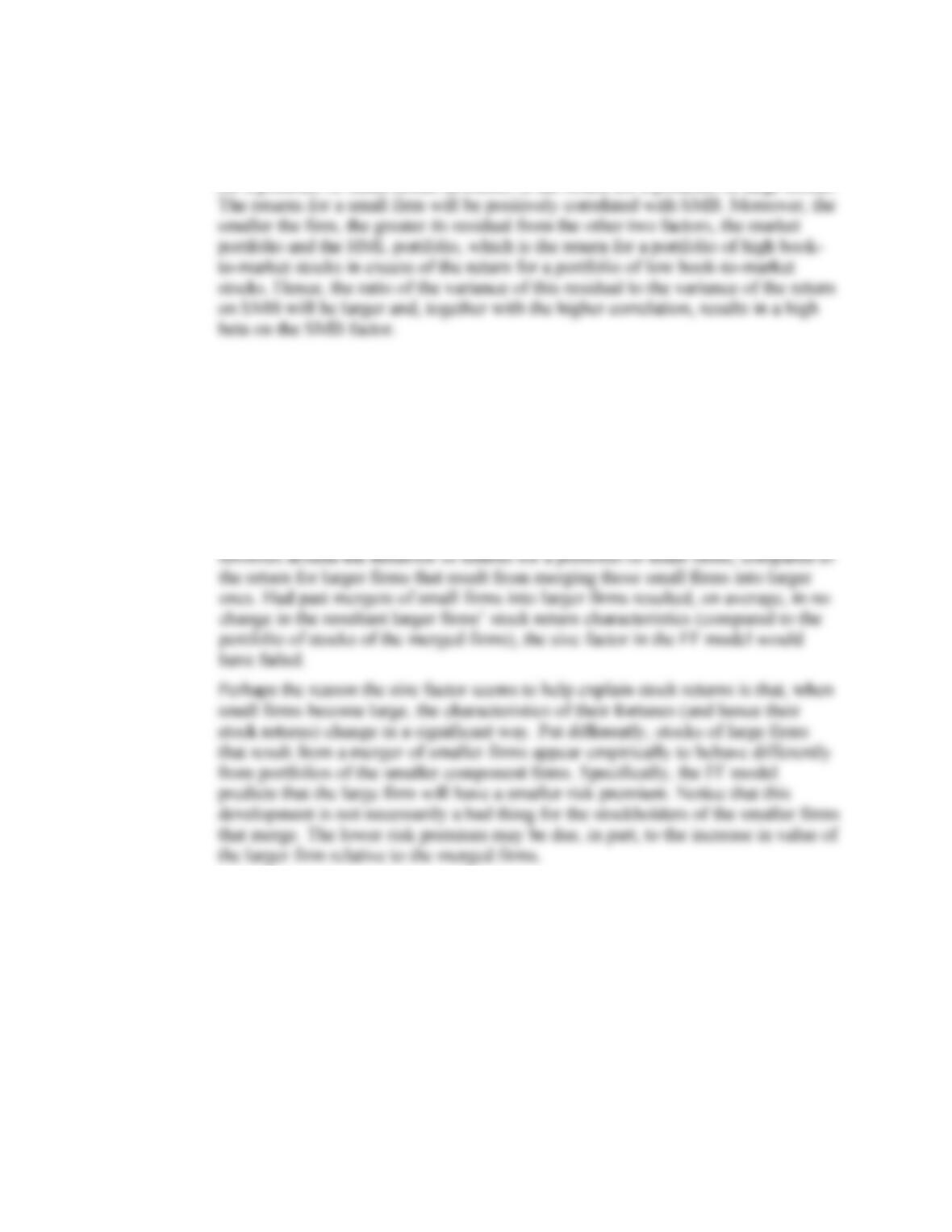
14. a. Assume a single-factor economy, with a factor risk premium EM and a (large) set
of well-diversified portfolios with beta P. Suppose we create a portfolio Z by
allocating the portion w to portfolio P and (1 – w) to the market portfolio M. The
rate of return on portfolio Z is:
RZ = (w × RP) + [(1 – w) × RM]
b. The same argument can be used to show that, in a three-factor model with factor
risk premiums EM, E1 and E2, in order to avoid arbitrage, we must have:
Chapter 10 – Arbitrage Pricing Theory and Multifactor Models of Risk and Return
10-7
15. a. The Fama-French (FF) three-factor model holds that one of the factors driving
returns is firm size. An index with returns highly correlated with firm size (i.e.,
firm capitalization) that captures this factor is SMB (Small Minus Big), the return
for a portfolio of small stocks in excess of the return for a portfolio of large stocks.
b. This question appears to point to a flaw in the FF model. The model predicts that
firm size affects average returns, so that, if two firms merge into a larger firm, then
the FF model predicts lower average returns for the merged firm. However, there
seems to be no reason for the merged firm to underperform the returns of the
component companies, assuming that the component firms were unrelated and that
they will now be operated independently. We might therefore expect that the
performance of the merged firm would be the same as the performance of a
portfolio of the originally independent firms, but the FF model predicts that the
increased firm size will result in lower average returns. Therefore, the question

Chapter 10 – Arbitrage Pricing Theory and Multifactor Models of Risk and Return
10-8
CFA PROBLEMS
1. a. This statement is incorrect. The CAPM requires a mean-variance efficient market
b. This statement is incorrect. The CAPM assumes normally distributed security
c. This statement is correct.
2. b. Since Portfolio X has = 1.0, then X is the market portfolio and E(RM) =16%.
6. c. Investors will take on as large a position as possible only if the mispricing