1
6 Increasing Returns to Scale and Imperfect Competition
Notes to Instructor
Chapter Summary
In the Ricardian and modified specific-factors model as well as in the Heckscher–Ohlin
model, we assumed perfectly competitive markets, where there are many firms, each
producing a homogeneous product, and where no firm is able to influence the market
price. In this chapter, we drop the assumption of perfectly competitive markets. We will
now assume imperfect competition, where firms are now able to influence the price of
their product.
This chapter focuses on the monopolistic competition model, where market power is
obtained through the ability to differentiate their product uniquely and thereby assume
some characteristics of a monopoly while retaining some characteristics of purely
competitive markets.
2
are a result of the two main characteristics of this model. The first characteristic is
product differentiation and the second feature is increasing returns to scale, where the
average costs for a firm fall as greater output is produced.
The first feature of product differentiation assumes firms are able to exert some control
over the price they can charge for their unique product. When firms produce
differentiated products, they retain some ability to set the price for their products without
risking the loss of all their business to competitors. Of course, they are not able to control
prices to the extent of a monopolist.
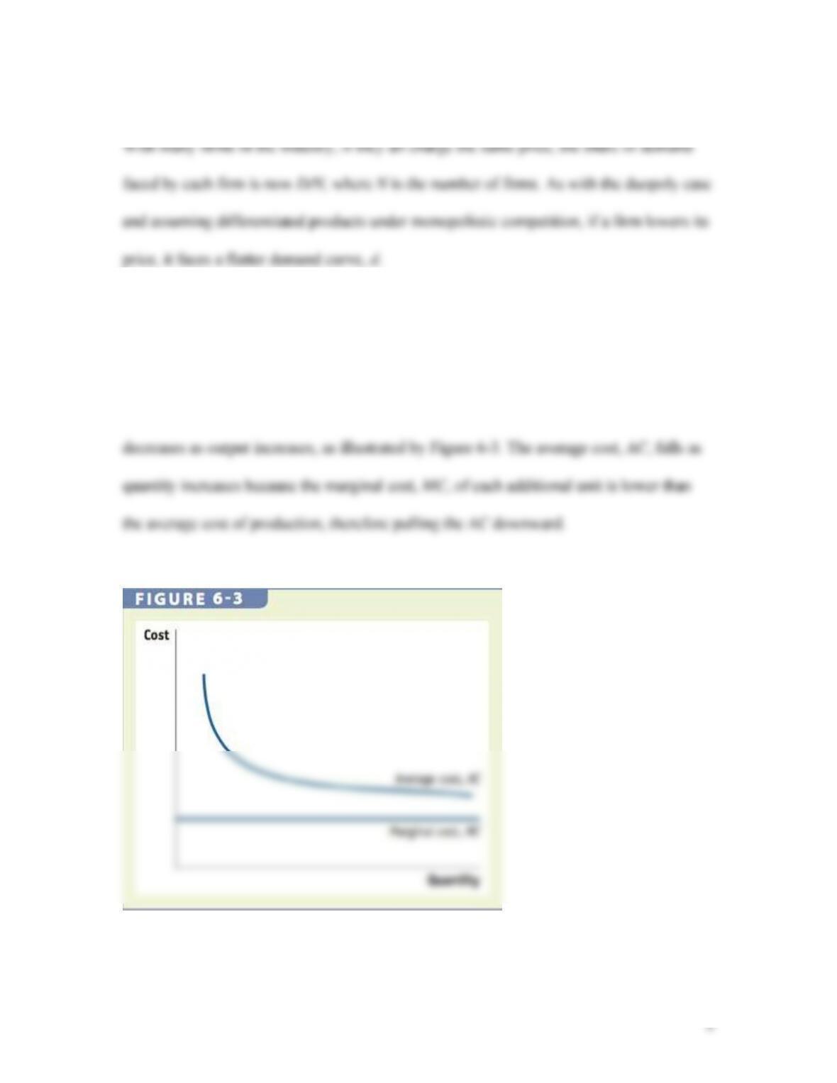
The second feature of monopolistic competition is increasing returns to scale. Here, firms
specialize in the product lines that are most successful, and by selling more of those
products, the average costs of production fall for them. Firms can lower their average
costs by selling not just in their own home markets but can achieve even lower costs by
selling in larger foreign markets, thereby increasing the size of the markets they reach.
So, increasing returns to scale create a reason for trade even in situations where trading
partners have similar technologies and similar factor endowments. Increasing returns to
3
Ocean, will be discussed in Chapter 11.
Comments
By now, students should have a good understanding of the concept of comparative
advantage as the basis for trade. To get them thinking about the monopolistic competition
model and product differentiation, find out how many prefer Coca Cola versus Pepsi
Lecture Notes
Introduction
Due to proximity, resources, and comparative advantage, the United States imported
4
snowboards from 20 different countries in 2009, although exporting very little in return.
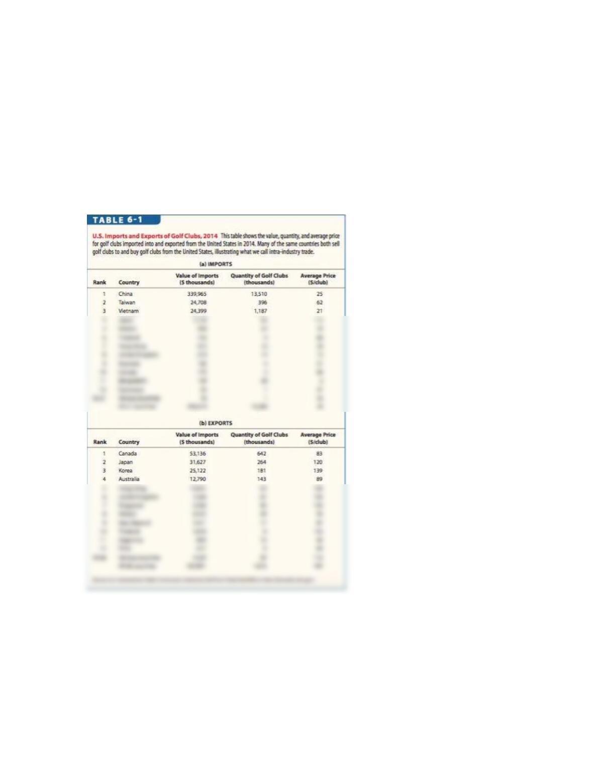
Now we illustrate why a country would buy a product from foreign countries and sell the
same product to them. In Table 6-1, we list the 12 countries that sell the most golf clubs
to the United States and the 12 countries to which the United States sells the most golf
clubs. The table also lists the amounts bought or sold and their average wholesale prices.
By contrast, the United States imported golf clubs valued at $399 million from 25
countries and exported $157 million of the product to about 66 countries in 2014. Panel
5
number 10 spot on the list of top U.S. -importing countries, it ranks number 1 among the
countries in which the United States exports golf clubs. Aside from Canada, four other
countries on the top importing list (Japan, the United Kingdom, Australia, and Hong
Kong) are also among the top 12 buyers of American golf clubs. The quality of golf clubs
exported from the United States, although higher than most of the clubs imported, also
endowment.
6
1 Basics of Imperfect Competition
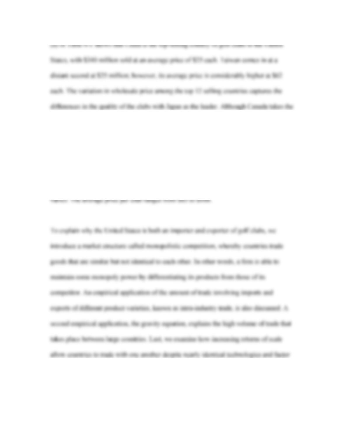
Monopoly Equilibrium We begin by reviewing the monopoly and duopoly market
cases. Understanding how demand is determined within these two types of markets will
help to explain how demand is determined in the monopolistic competitive market.
Recall from your principles course that as the sole producer in a market, the demand
curve faced by the monopolist is the industry demand curve. As shown in Figure 6-1, the
7
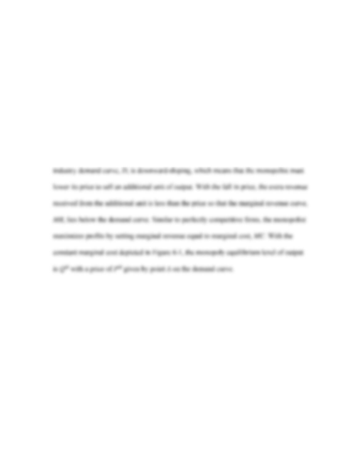
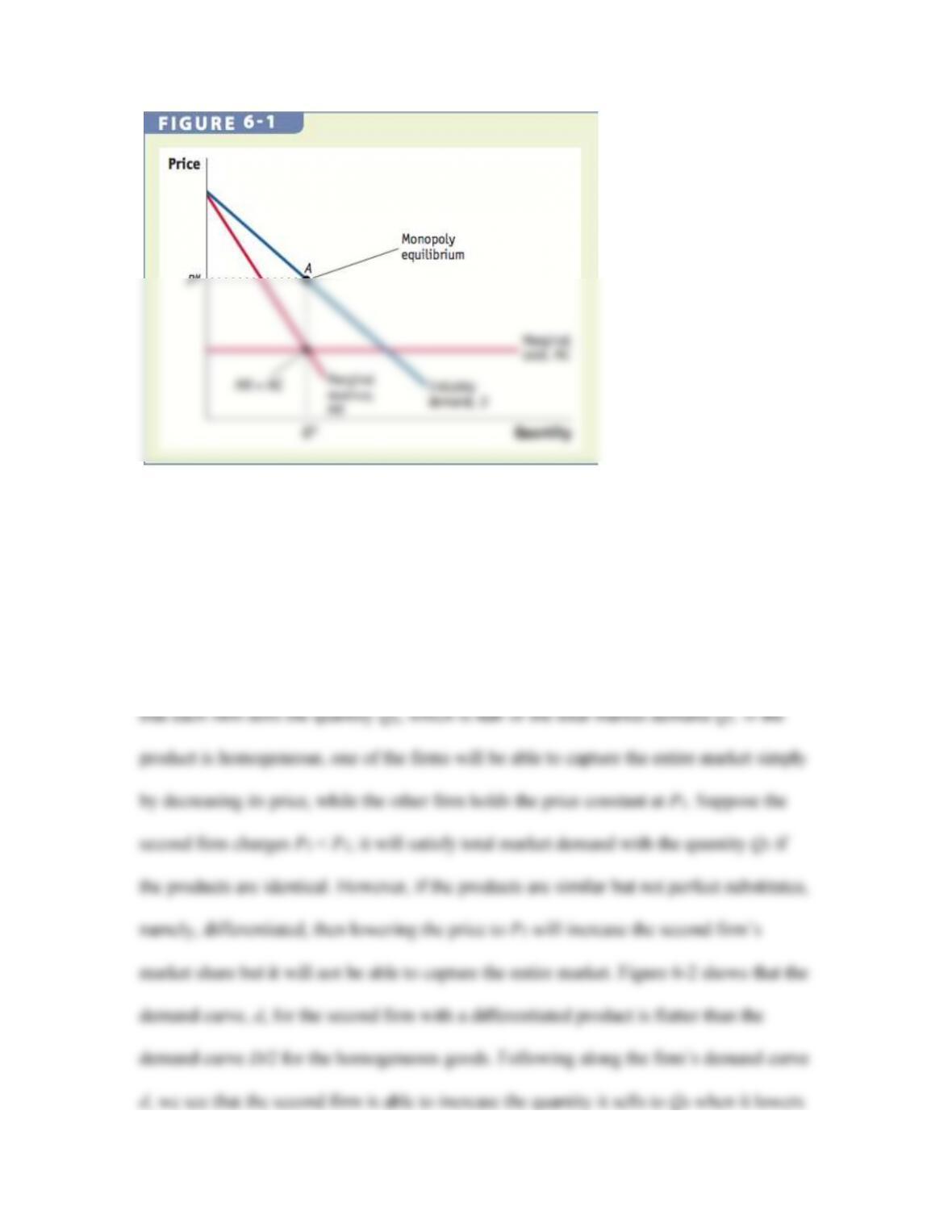
Demand with Duopoly By adding one additional firm to the industry, we have a
duopoly, where the industry demand curve, D (illustrated in Figure 6–2), is shared
between the two competitors. If they charge identical prices, each firm faces one half of
the industry demand, D/2. Namely, at the price of P1, the industry demand is at point A so
8
the price to P2 if the first firm maintains its price at P1.
2 Trade Under Monopolistic Competition
We will now turn to the monopolistic competition model beginning with assumption 1.
Assumption 1: Each firm produces a good that is similar to but differentiated from the
goods that other firms in the industry produce.
Assumption 2: There are many firms in the industry.
Assumption 3: Firms produce using a technology with increasing returns to scale.
Increasing returns to scale technology means that the average cost of production
10
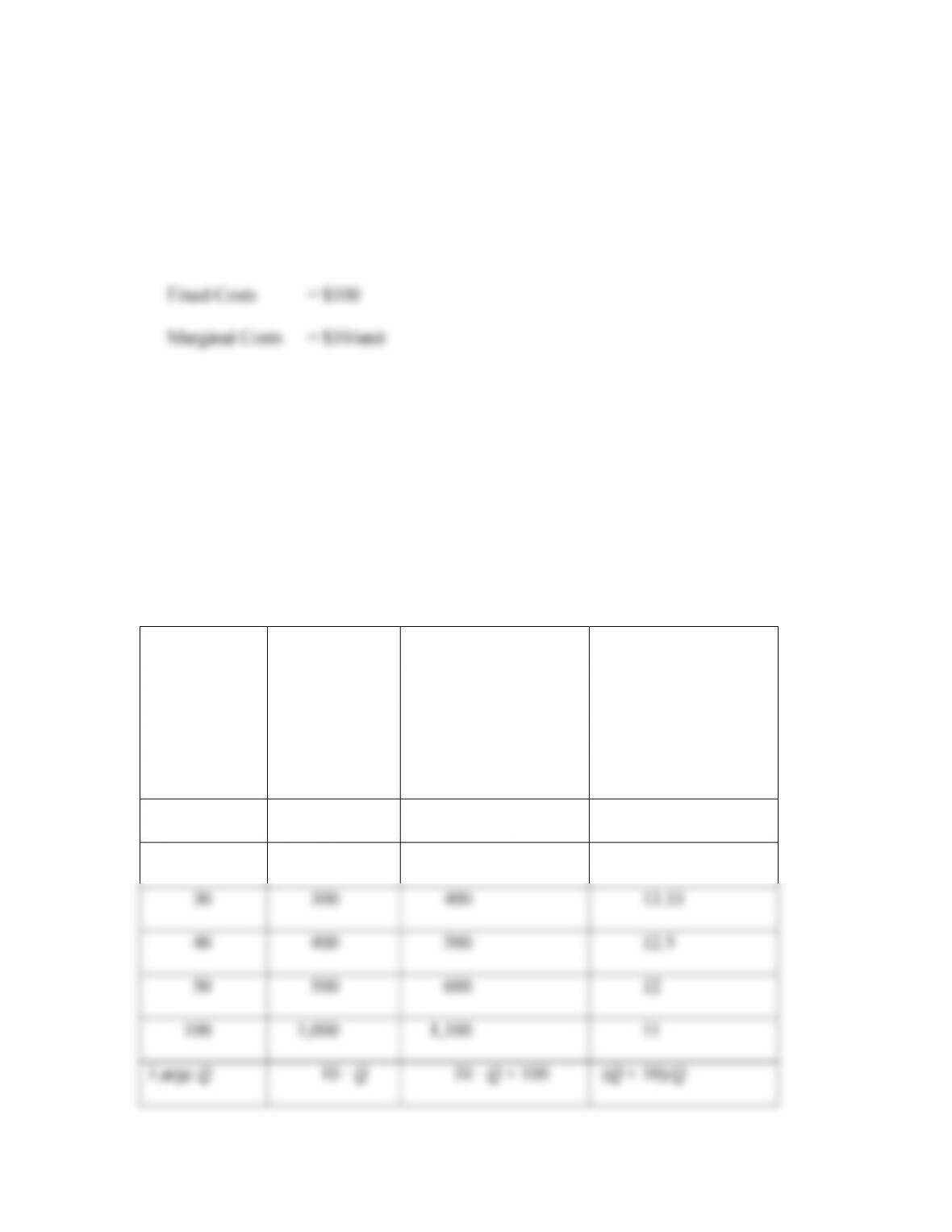
Numerical Example For simplicity, let’s look at a numerical example with a firm that
has constant marginal costs similar to those depicted in Figure 6-3. Suppose the firm has
the following costs of production:
From the following table, we see that average cost for the first ten units of output is $20
each. Notice that marginal cost is lower at $10 per unit. Because MC is less than AC, the
firm would be able to lower its average costs by increasing the quantity produced. With
the next additional 10 units produced, the firm’s AC decreases to $15 per unit.
Quantity, Q
Variable costs
= Q • MC
Total Costs =
Variable Costs+
Fixed Costs (FC =
$100)
Average Costs =
Total Costs/Quantity
10
$100
$200
20
20
200
300
15
30
300
400
13.33
40
400
500
12.5
50
500
600
12
100
1,000
1,100
11
Large Q
10 · Q
10 · Q + 100
(Q + 10)/Q
11
(close to 10)
Assumption 4: Firms can enter and exit the industry freely, so monopoly profits are zero
in the long run.
Equilibrium Without Trade
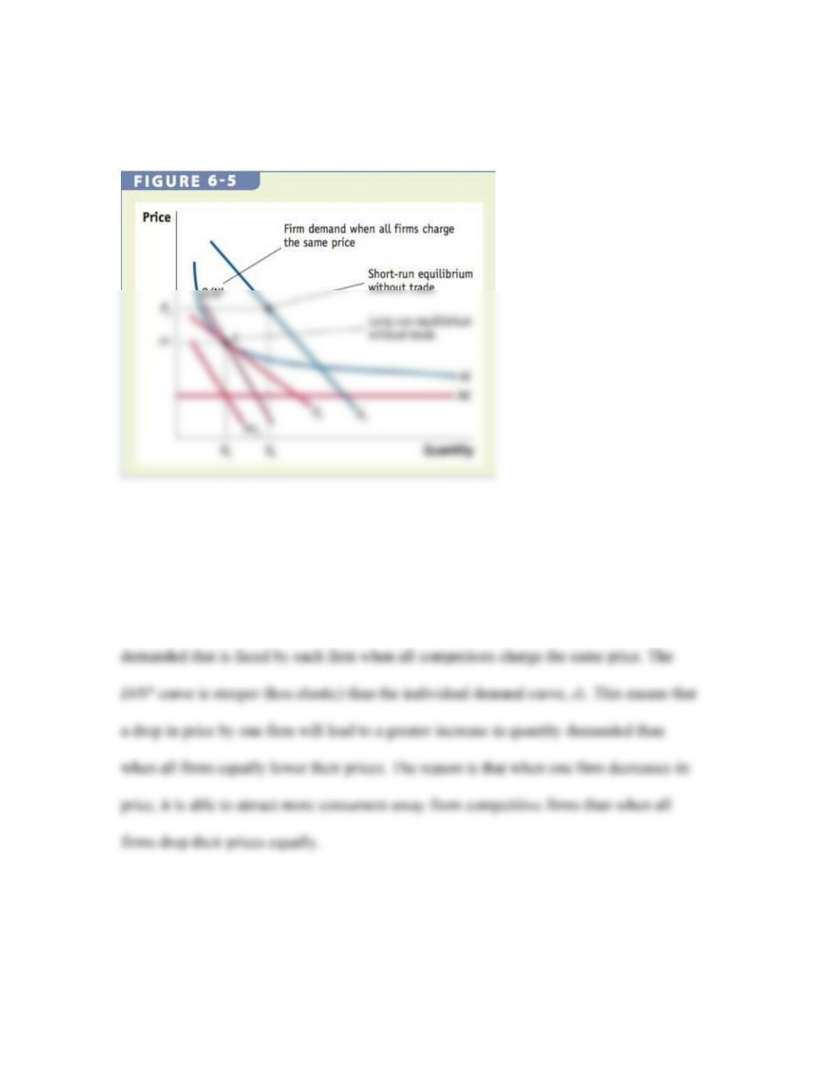
Short–Run Equilibrium As shown in Figure 6-4, a firm in a monopolistic competition
faces a downward-sloping demand curve, d0. This is because consumers view its product
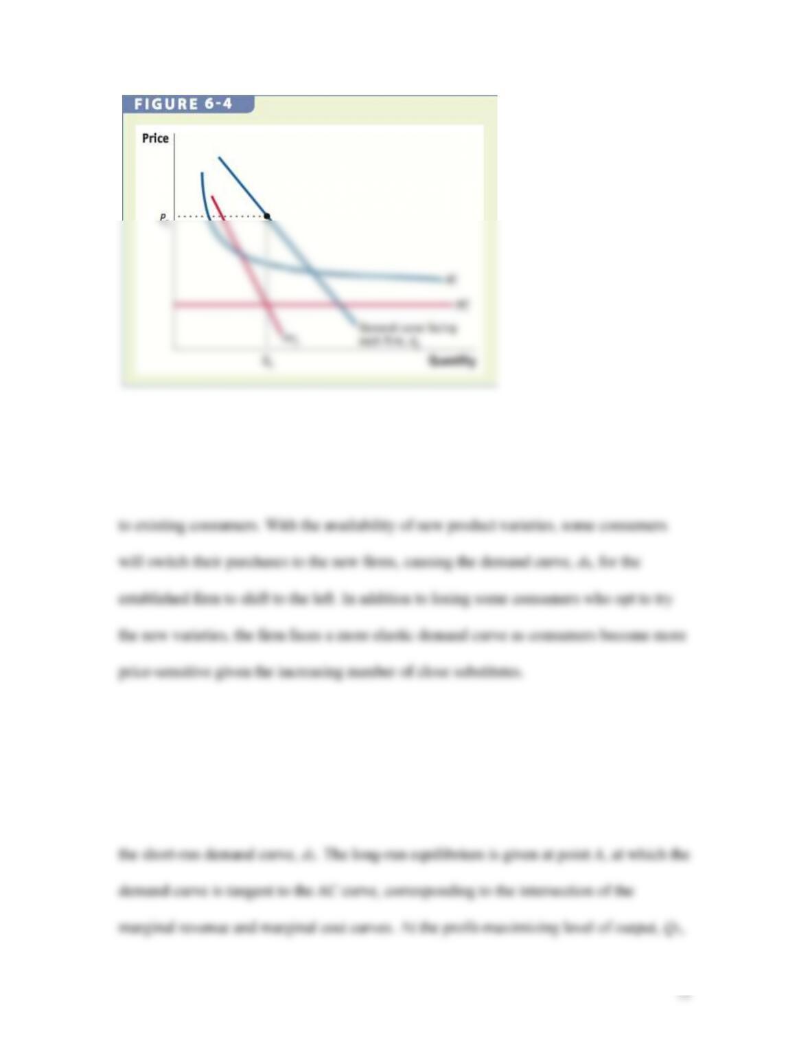
12
Long–Run Equilibrium Attracted by the monopoly profits and given the assumption of
free entry into the industry, new firms will provide similar, albeit not identical, products
Entry by new firms continues until all positive monopoly profits are exhausted. At this
point, the industry is in a long-run equilibrium, where firms neither want to enter nor exit.
Illustrated by Figure 6-5, the demand curve, d1, in the long run is flatter and to the left of
13
and price, PA, the firm is making zero profits because price equals average costs.
We now introduce another demand curve, D/NA, to Figure 6-5 before examining trade
under monopolistic competition. This demand curve, derived from dividing the total
market demand, D, by the number of firms in autarky, NA, reflects the quantity that
Equilibrium with Free Trade
Suppose firms in both Home and Foreign are monopolistically competitive. For
14
simplicity, further assume that the two countries are identical in terms of size, number of
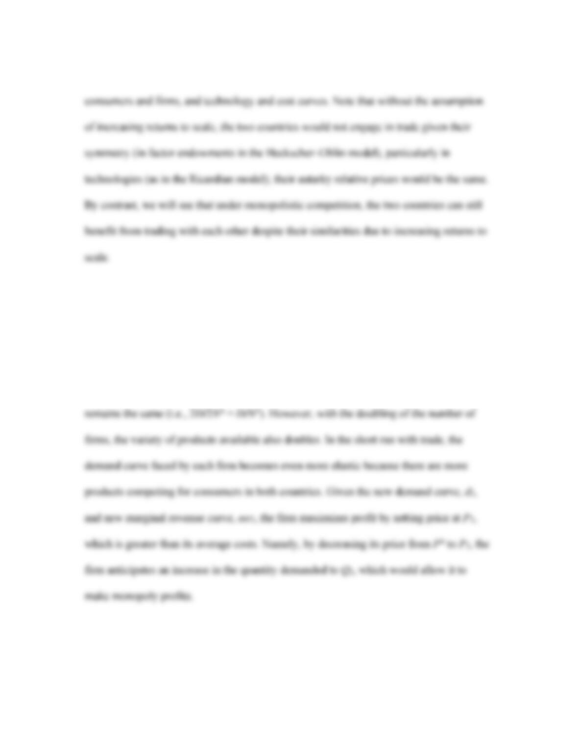
Short–Run Equilibrium with Trade We begin with the no-trade equilibrium given by
point A in Figure 6-5, which is reproduced in Figure 6-6. As the two countries engage in
trade, the number of consumers each firm can serve doubles. Likewise, there are twice as
many firms available to consumers in each country so that the demand curve, D/NA,
However, motivated by the same incentive to attract consumers from other firms by
15
lowering prices, every firm in the industry will make the same decision. This collective
move means that the quantity demanded for any one firm does not increase along the
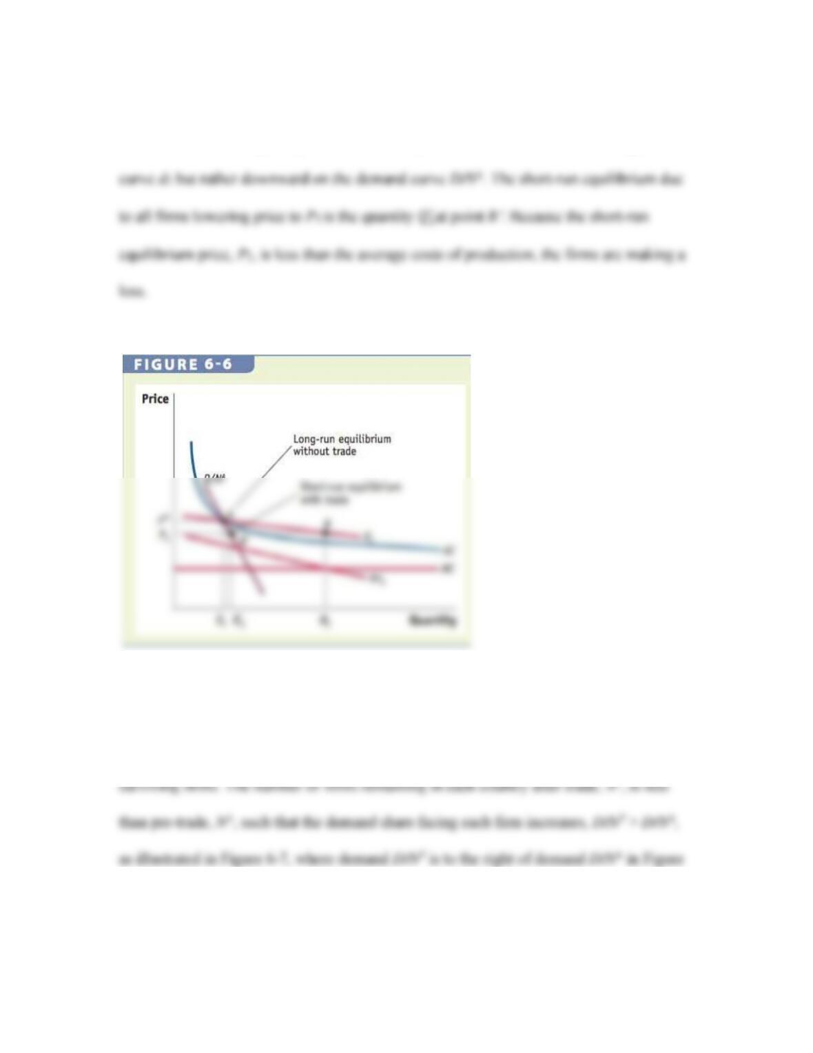
Long–Run Equilibrium with Trade The losses will cause some firms to leave the
industry, reducing the product varieties available to consumers and increasing demand for
6-6. Although there are fewer firms than before trade, the number of products available to
consumers in each country has increased, that is, 2NT > NA. Given the availability of
16
greater product variety with trade, the demand curve, d3, facing each firm is more elastic
than with absence of trade. The intersection of the marginal revenue curve, mr3, with the
marginal cost curve gives the long-run equilibrium with trade at point C, where all firms
Gains from Trade In general, consumers gain as a result of trade under monopolistic
competition. In particular, consumers benefit because of the reduction in the price, as
reflected by the increasing returns to scale the firms remaining in the industry receive.
Adjustment Costs from Trade Nevertheless, to fully examine the overall effect of trade
when firms compete under imperfect competition, we need to also analyze the short-run
3 The North American Free Trade Agreement
Although the notion that trade could lead to an increase in product varieties was
Gains and Adjustment Costs for Canada Under NAFTA
The gains and losses for Canada after joining the Canada–U. S. Free Trade Agreement
(CUSFTA) were examined by economist Daniel Trefler at the University of Toronto.
18
regional agreement amount to a 5% loss of employment in manufacturing, or about
100,000 jobs. These losses, however, were compensated by employment created in other
parts of the industry over time.
Trefler also estimated that the industries most affected by the tariff cuts experienced an
increase in productivity rising as much as 18% over 8 years within the industries most
affected by tariff cuts. This reflects a compound growth rate of 2.1% per year.
Manufacturing itself experienced a compound growth rate in productivity of 0.7%. The
difference between 2.1 − 0.7 = 1.4% provides an estimate of how free trade with the
United States impacted the Canadian industries most affected by the tariff cuts over and
above the impact on other industries.
However, real earnings in Canada rose by a modest 2.4% for production workers or .3%
per year in spite of the 0.7% per year in productivity growth in manufacturing, suggesting
that perhaps manufacturing workers did not entirely share in the gains from productivity.
Gains and Adjustment Costs for Mexico Under NAFTA
As part of its economic reforms, Mexico joined NAFTA along with the United States and
Canada in 1994. Under NAFTA, Mexican tariffs on U.S. goods declined from 14% in
H E A D L I N E S
Nearly 20 Years After NAFTA, First Mexican Truck Arrives in U.S. Interior
On October 21, 2011, the first big-rig truck from Mexico crossed the border into Laredo,
Texas, under a trucking program that was agreed to in NAFTA, but took nearly 20 years
to implement. The Obama administration finally signed an agreement with Mexico to end
Productivity in Mexico We can examine the growth in labor productivity in Mexico, as
shown in panel (a) of Figure 6-8 for maquiladora plants—those near the U.S. border,
producing mostly for export to United States—and for all other non-maquiladora
manufacturing plants. From 1994 to 2003, the labor productivity increased by 45% and
25% in maquiladora and non-maquiladora plants, respectively.
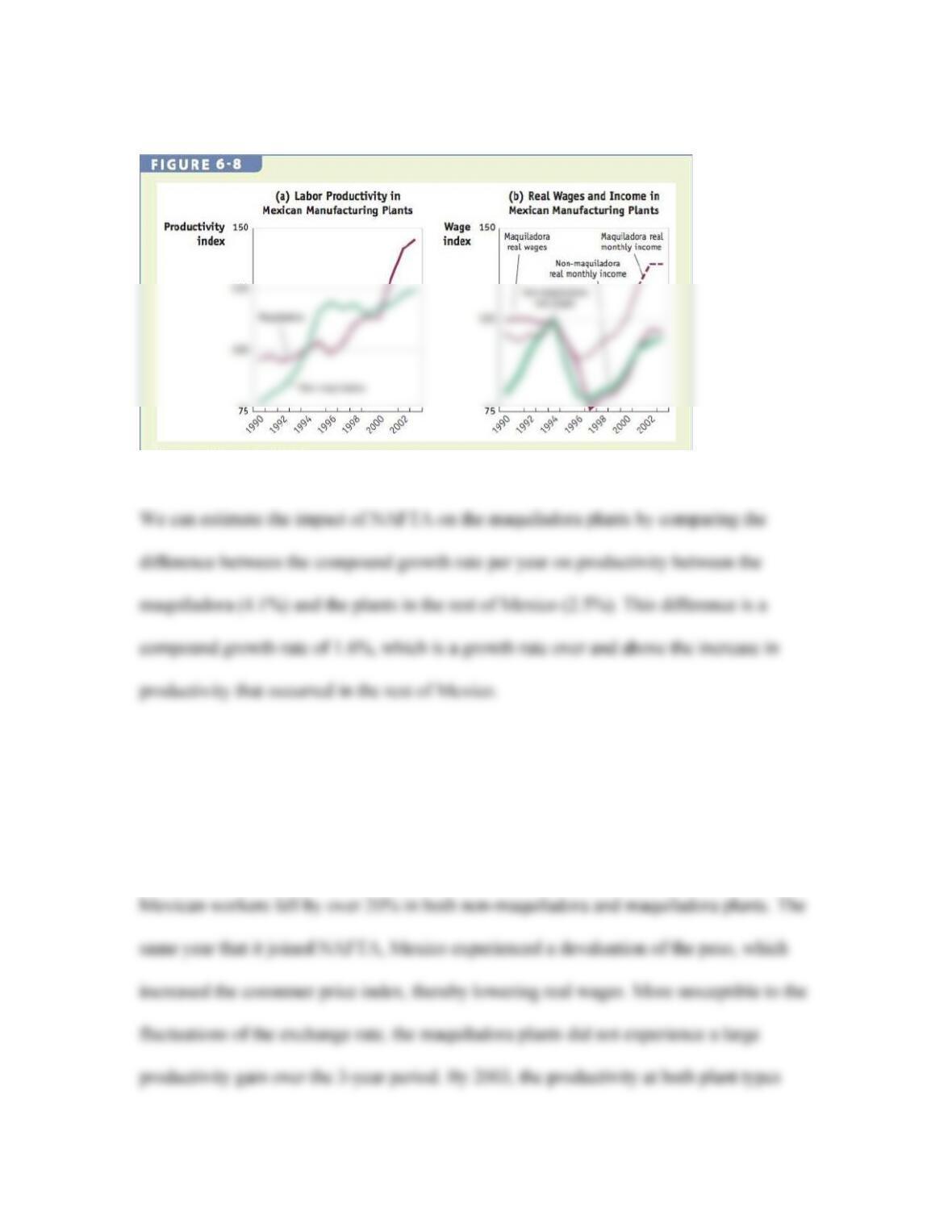
20
Real Wages and Incomes Panel (b) of Figure 6–8 shows the real wages in the
maquiladora and non-maquiladora plants. Between 1994 and 1997, the real wages for