rose over 20% relative to the level in 1994. In both sectors, real wages increased by 2003
to the levels reached in 1994.
As an alternative to examining real wages, we could instead study the real monthly
income, which would more accurately reflect the earnings of higher-income individuals
Adjustment Costs in Mexico
Before NAFTA, it was expected that Mexico’s agricultural sector, particularly corn
growers, would face severe short-run adjustment costs due to intense import competition
from the United States. Post-NAFTA, there is no evidence that Mexican corn growers
22
Within the manufacturing maquiladora sector, employment grew post-NAFTA from
584,000 workers in 1994 to a height of 1.29 million workers in 2000. However, as a
It is difficult to determine whether this roller coaster ride in employment was a result of
NAFTA short-run adjustment costs or the deleterious macroeconomic milieu the country
Gains and Adjustment Costs for the United States Under NAFTA
To examine the gains and losses in the United States from the entry of its southern
neighbor into the free-trade agreement, we begin by noting that consumers, as well as
23
This topic has been hotly debated in the United States, where it has been argued that
NAFTA would result in a “giant sucking sound” of manufacturing plants leaving the
H E A D L I N E S
Opposing Viewpoints on the Effect of NAFTA, 20 Years Later
There have been differing viewpoints with regard to the benefits and costs of the NAFTA
trade agreement. We have provided two editorials here that take opposing positions
regarding the costs and benefits.
24
Institute for International Economics, outlines these benefits, such as consumer gains
from lower prices and the potential for job creation in the United States as U.S.
Expansion of Variety to the United States It was expected that one of the gains from
NAFTA would be lower prices of products, but such a plus can be very challenging to
measure. So, in this section, we will discuss the other important gain that may be
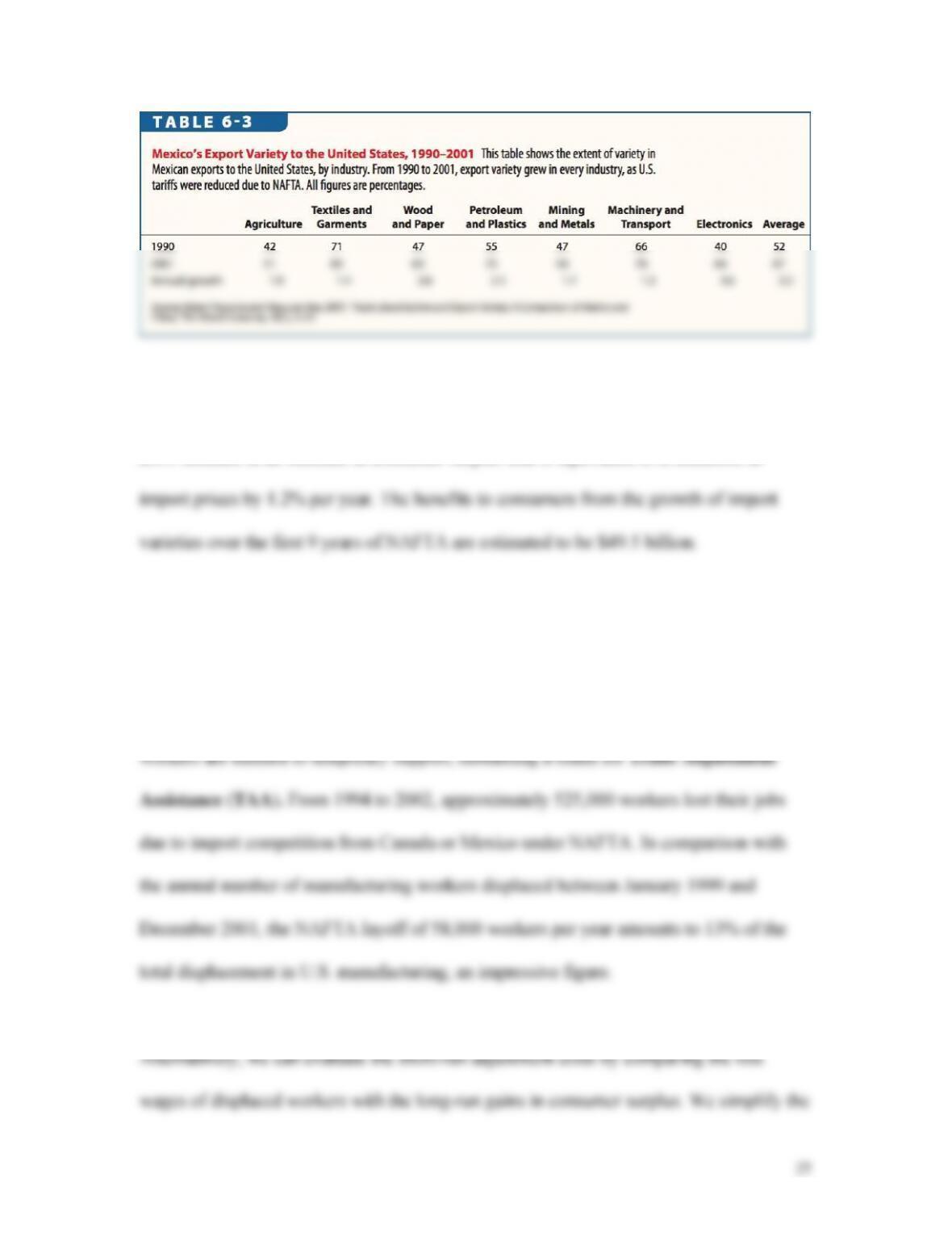
25
In addition to Mexico, the rise in product varieties from all countries between 1972 and
2001 resulted in an increase in consumer surplus that is equivalent to a reduction in
Adjustment Costs in the United States Short-run adjustment costs consist of the exiting
of domestic firms due to foreign competition. As firms leave the manufacturing industry,
workers become temporarily unemployed. Under U.S. trade laws, these displaced
26
Multiplying the average yearly earning in manufacturing in 2000 ($31,000) by 3, we see
that the wage lost due to displacement is $93,000 per worker. It follows that the annual
Summary of NAFTA The long-run gains to the United States come from the expansion
of product varieties from Mexico as well as the drop in consumer prices that come from
In terms of the United States and Canada, the long-run gains are greater than the short-
27
workers in the maquiladora sector since they experienced a rise in their real earnings.
Intra–Industry Trade and the Gravity Equation
In the Ricardian and Heckscher‒Ohlin models, countries traded homogeneous goods
either by exporting or importing the products but not both. But under the monopolistic
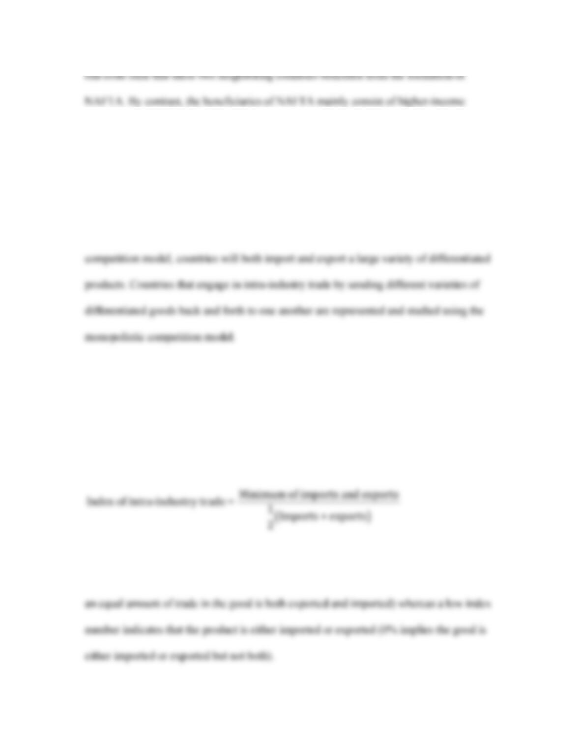
Index of Intra–Industry Trade To determine what proportion of a good traded involves
both imports and exports, we calculate the index of intra–industry trade given by the
following equation:
( )
Minimum of imports and exports
Index of intra-industry trade = 1Imports + exports
2
A high index indicates that trade involves both imports and exports. (100% implies that
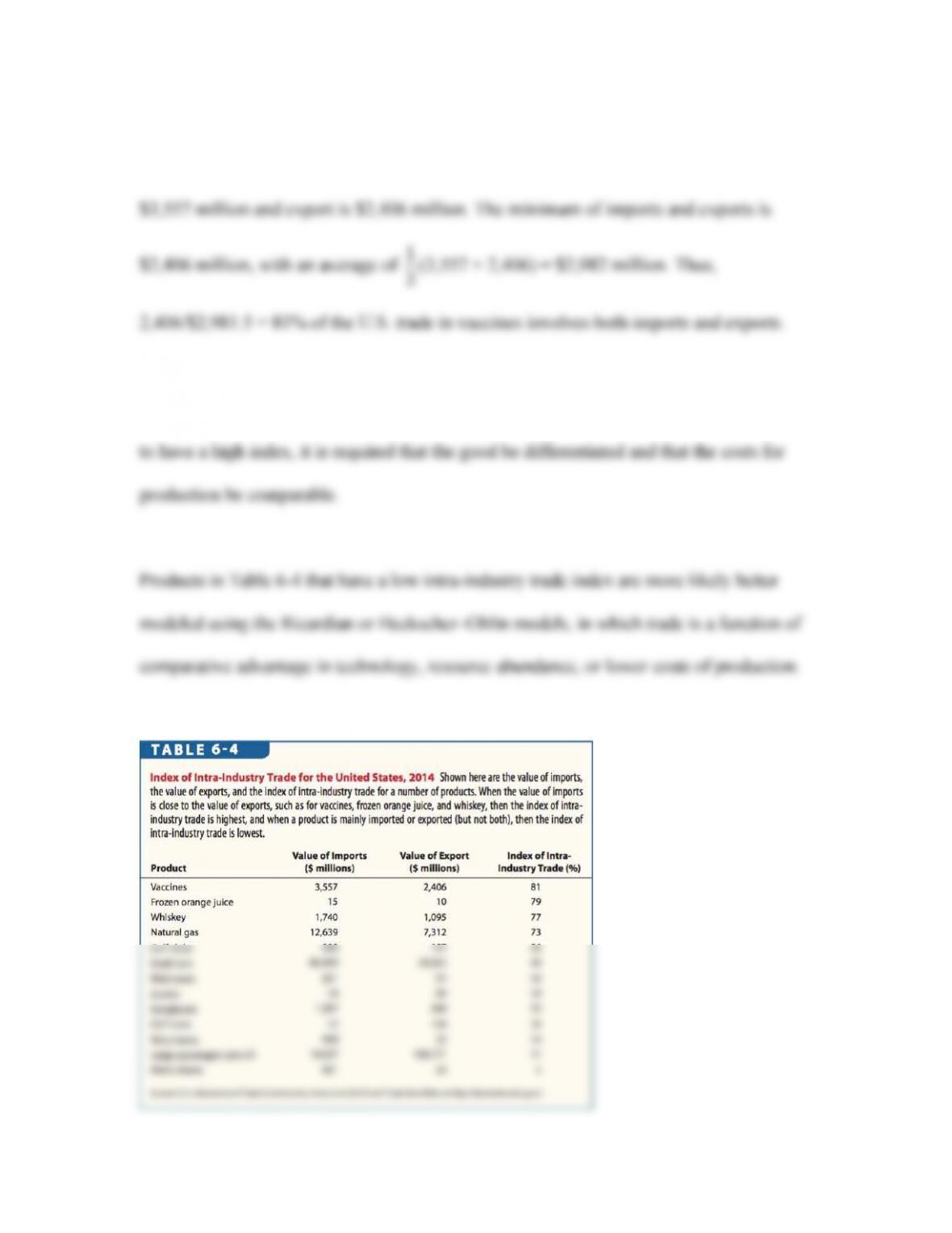
28
As an example, we use the information that the value of import for vaccines in 2014 is
Table 6–4 shows other examples of intra-industry trade in the United States. For products
29
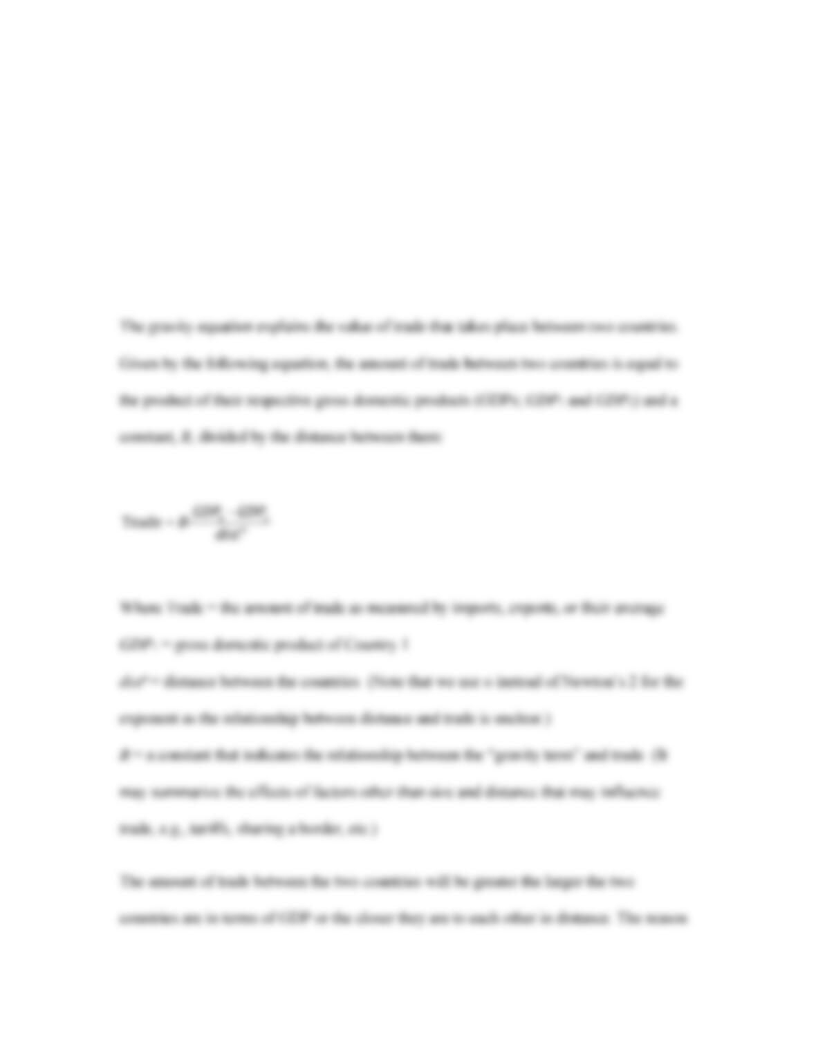
The Gravity Equation
The Gravity Equation in Trade The weakness of the intra-industry trade index is that it
fails to inform us of the total amount of trade between nations. The gravity equation will
be used for this purpose.
12
·
Trade = · n
GDP GDP
B
dist
Where Trade = the amount of trade as measured by imports, exports, or their average
GDP1 = gross domestic product of Country 1
distn = distance between the countries (Note that we use n instead of Newton’s 2 for the
exponent as the relationship between distance and trade is unclear.)
B = a constant that indicates the relationship between the “gravity term” and trade (It
may summarize the effects of factors other than size and distance that may influence
trade, e.g., tariffs, sharing a border, etc.)
The amount of trade between the two countries will be greater the larger the two
countries are in terms of GDP or the closer they are to each other in distance. The reason
30
Deriving the Gravity Equation To derive the gravity equation, we assume each country
produces a differentiated product to apply the monopolistic competition model. With a
differentiated product, the import demand for goods produced by Country 1 depends on
=
1 2 12
· ·
1
Trade = nn
W
GDP Share GDP GDP
dist GDP dist
By denoting the term (1/GDPW) as a constant term, B, we have the gravity equation.
APPLICATION
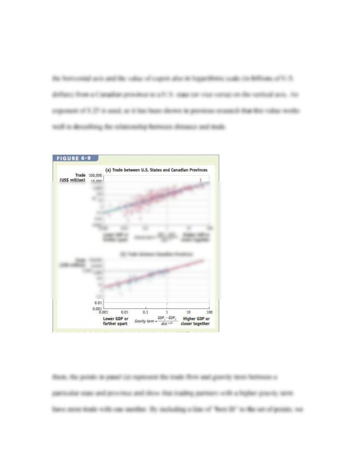
The Gravity Equation for Canada and the United States
The gravity equation may be applied between countries, provinces, or even states of a
31
country. Panel (a) of Figure 6–9 shows the trade between U.S. states and Canadian
provinces in 1993 with the gravity term (= GDP1GDP2/dist1.25) as a logarithmic scale on
With data from 30 states and 10 provinces and a total of 600 possible trade flows between
32
Trade Within Canada
The gravity equation can also predict intra-national trade, or trade within a country as
well. Panel (b) of Figure 6-9 shows the value of exports between pairs of Canadian
Comparing the gravity equation for international trade with intra–national trade, we find a
much larger term of 1,300 compared with the 93. The ratio of the two (1,300/93 = 14)
indicates that trade among the provinces is 14 times greater than that between Canada and
33
5 Conclusions
In contrast to classical trade models such as the Ricardian model and the Heckscher‒
Ohlin model, we find that two seemingly identical countries can benefit from trading with
one another when we remove the assumption of perfect competition. Under monopolistic
Despite potential for long-term gains to consumers in the form of lower prices and
increased variety and to remaining producers from greater efficiency, a comparison of the
34
agreements.
TEACHING TIPS
Tip 1: Understanding Increasing Returns to Scale and Monopolistic Competition
Chapter 6 introduces a very important, but difficult, model of trade. For students to
understand the complexity of this model, it is imperative that they fully grasp the
Tip 2: Adjustment Costs and Trade Adjustment Assistance
In the model of Chapter 6, trade creates a firm exit, which results in short–term costs to
trade. Ask students to independently research the changes made to the Trade Adjustment
Tip 3: Data Analysis of Intra-Industry Trade
We continue our effort to familiarize students with economic data by asking
students to investigate the level of intra-industry trade for goods of their own
35
choosing. Ask students to look up the Harmonized Tariff code (HTC) for four goods,
IN–CLASS PROBLEMS
1. How does increasing returns to scale lead to gains from trade under monopolistic
competition?
Answer: Through trade, firms are able to expand their outputs by selling in the
Foreign market. With the rise in the number of product varieties available,
2. Portland and Aleland are two identical countries. Beer manufacturers in each country
compete under monopolistic competition.
a. Suppose the two countries engage in trade. Determine the impact of free trade on
consumers in Portland.
b. How does trade affect the welfare of domestic producers in Portland?
Answer: By selling abroad, the producers in Portland will be able to lower their
3. What had Canada expected to gain from forming the CUSFTA with the United
States?
Answer: Relative to the United States, the Canadian market is small. By forming
4. Refer to the gravity equation.
a. Why is trade greater between two large trading partners?
37
b. How does distance between trading partners influence the amount of trade?
5. In the monopolistic competition model, would you expect prices to be higher or lower
as the number of firms increases? Briefly explain why.
6. Assume a firm has the following costs:
Fixed costs: $100
Marginal costs: $50/unit
a. Fill in the missing information on the following chart:
Quantity, Q
Variable
Total Costs =
Average Costs =
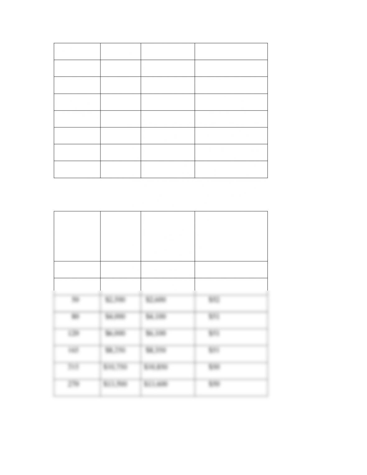
38
5
25
50
80
120
165
215
270
Answer:
Quantity, Q
Variable
costs = Q ·
MC
Total Costs =
Variable Costs
+ Fixed Costs
Average Costs =
Total Costs/Quantity
5
$250
$350
$70
25
$1,250
$1,350
$54
50
$2,500
$2,600
$52
80
$4,000
$4,100
$51
120
$6,000
$6,100
$51
165
$8,250
$8,350
$51
215
$10,750
$10,850
$50
270
$13,500
$13,600
$50
b. At what level of output does the firm experience increasing returns to scale?
39
7. How does an increase in the number of product varieties benefit an importing
country?
Answer: Assuming that consumers prefer more varieties to less, an increase in the