4 Trade and Resources: The Heckscher–Ohlin Model
Notes to Instructor
Chapter Summary
This chapter presents the Heckscher–Ohlin model with two factors (capital and labor),
two goods (computers and shoes), and two countries (Home and Foreign). A test of the
model is discussed with Leontief ’s paradox. Additionally this chapter, like the last,
discusses the affect of trade on factor prices. The “sign test” in the Heckscher-Ohlin
model is discussed in the Appendix.
Comments
Note that this chapter covers only two theorems of the Heckscher–Ohlin model—the
Heckscher–Ohlin theorem and the Stolper–Samuelson theorem. The other two
theorems—the Rybczynski theorem and Factor Price Insensitivity—are deferred to the
next chapter, in an effort to break the material into smaller pieces.
Unlike the previous chapters, a discussion of the theory is followed by an empirical
test. This concept is possibly new to students and could be highlighted to generate
Lecture Notes
Introduction
We begin the chapter with a comparison between the Ricardian model, in which trade
occurs due to differences in technology between countries giving rise to their
1 Heckscher–Ohlin Model
The Heckscher-Ohlin model consists of two factors (capital and labor), two goods
(computers and shoes), and two countries (Home and Foreign). The total amount of
Assumptions of the Heckscher–Ohlin Model
The six assumptions of the Heckscher–Ohlin model are as follows:
Assumption 1: Both factors can move freely between the industries.
The implication of the first assumption is that the rental on capital, R, is identical
across the two industries. If one industry has a higher rental, it would attract capital from
Assumption 2: Shoe production is labor-intensive, that is, it requires more labor per unit
of capital to produce shoes than computers, so that LS/KS > LC/KC.
The second assumption states how intensive the factors are in the production of each
good. Namely, computer production is capital-intensive, requiring more capital per
[FIGURE 4–1 MISSING FROM PDF TEXT]
Assumption 3: Foreign is labor-abundant, by which we mean that the labor–capital ratio
in Foreign exceeds that in Home, . Equivalently, Home is capital
Assumption 4: The final outputs, shoes and computers, can be traded internationally, but
labor and capital do not move between countries.
The assumption allows the final goods to move between the countries but not the
factors of production.
Assumption 5: The technologies used to produce the two goods are identical across the
countries.
From the fifth assumption, we see that each good is produced using the same
Assumption 6: Consumer tastes are the same across countries, and preferences for
computers and shoes do not vary with a country’s level of income.
APPLICATION
Are Factor Intensities the Same Across Countries?
In the United States, footwear production is more capital-intensive than call centers
because of the expensive automated–manufacturing machines used by a New Balance
plant. However, there is a “reversal” of factor intensities in India, where call centers are
N E T W O R K
The New Balance website can be found through the following link:
No–Trade Equilibrium
Production Possibility Frontiers Figure 4-2 shows the production possibility frontiers
(PPFs) for Home in panel (a) and Foreign in panel (b). The bowed-out PPF is biased
toward computer (on the horizontal axis) for Home because Home is capital-abundant
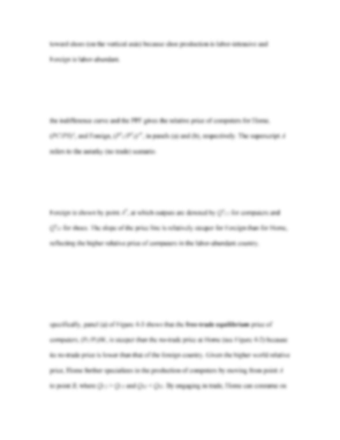
Indifference Curves With the assumption of common consumer tastes across the
countries, we add an identical indifference curve to each country’s PPF. The tangency of
No–Trade Equilibrium Price The no–trade equilibrium for Home is at point A, with
production of computers and shoes given by QC1 and QS1. The no-trade equilibrium for
Free–Trade Equilibrium
Home Equilibrium with Free Trade With free trade, the equilibrium relative price of
computers is between the no-trade relative prices found at Home and Foreign. More
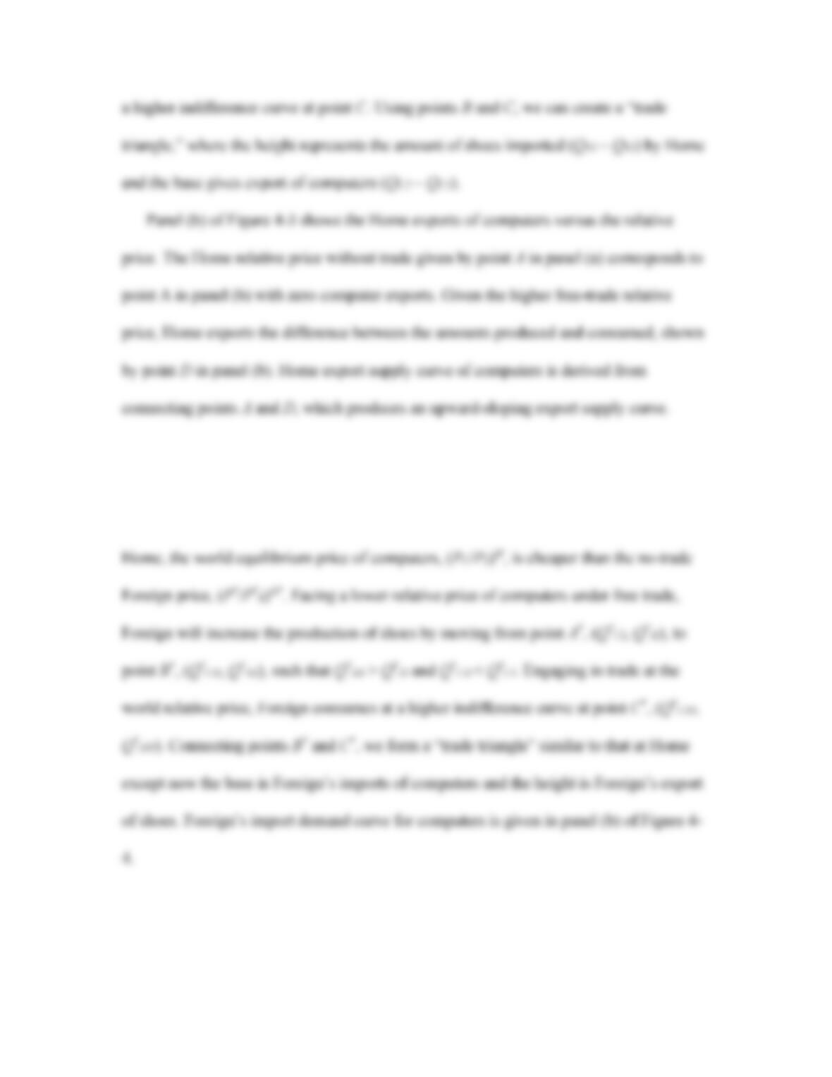
Foreign Equilibrium with Free Trade In panel (a) of Figure 4-4, the Foreign no-trade
equilibrium is at point A*. Because the Foreign no–trade relative price is higher than at
Equilibrium Price with Free Trade Putting together Home’s export supply curve for

computers and Foreign’s import demand curve for computers gives the equilibrium
Pattern of Trade The pattern of trade can be determined from the free–trade equilibrium.
Namely, a country will export the good that uses intensively the factor of which it has an
Heckscher–Ohlin Theorem With two goods and two factors, each country will export
2 Testing the Heckscher–Ohlin Model
Testing the Heckscher–Ohlin Theorem: Leontief’s Paradox
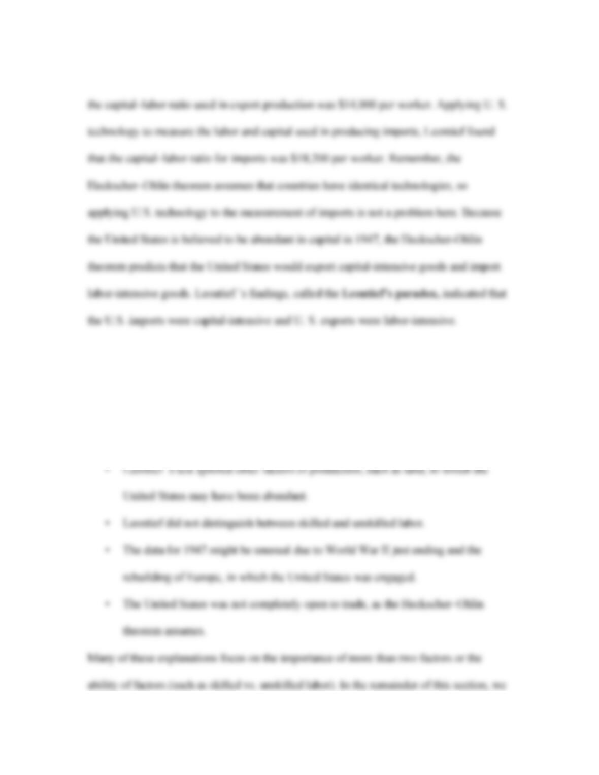
required to produce $1 million worth of U. S. exports. The measurement indicated that
Explanations Many explanations have been offered to explain Leontief ’s paradox,
including the following:
• Technologies in the United States and rest of the world may not have been the
same as the Heckscher–Ohlin theorem assumes.
complexities.
Endowments in the New Millennium
The method for measuring factor abundance differs when we consider more than two
factors of production. The general definition of factor abundance is given by the
Capital Abundance Using the general definition and data from Figure 4-6, we see that in
2013 the United States was physical–capital scarce because its share of the world’s capital
Labor and Land Abundance Using a similar comparison, Figure 4-6 shows that the
United States is abundant in research and development (R&D) scientists and skilled
Differing Productivities Across Countries
Although the extended Heckscher–Ohlin model is better at predicting the pattern of
Measuring Factor Abundance Once Again Measuring whether a country is abundant
in that effective factor or scarce in that effective factor is similar to the method we
used earlier except that we now compare its share of the effective factor endowment,
Effective R&D Scientists To account for the differences in productivities across
countries due to the availability of laboratory equipment, we measure effective R&D
scientists by multiplying the actual number of R&D scientists by the amount of R&D
Effective Arable Land The effective amount of arable land is defined as the actual
arable land in a country times its productivity in agriculture. After accounting for the
differing productivities in arable land, we find that the U.S. was abundant in effective
H E A D L I N E S
China Drawing High–Tech Research from the United States
Applied Materials, a U.S. firm that is currently the world’s largest supplier of equipment
used to make semiconductors, has built its newest and largest research labs in Beijing and
Leontif’s Paradox Once Again
Going back to data from the time periods studied by Leontief, with our newly developed
concepts of effective abundance, we can redo Leontief ’s factor calculations, taking into
solving Leontief ’s paradox.
3 Effects of Trade on Factor Prices
In this section, we determine the impact of trade on the wage and rental earned by labor
Effect of Trade on the Wage and Rental of Home
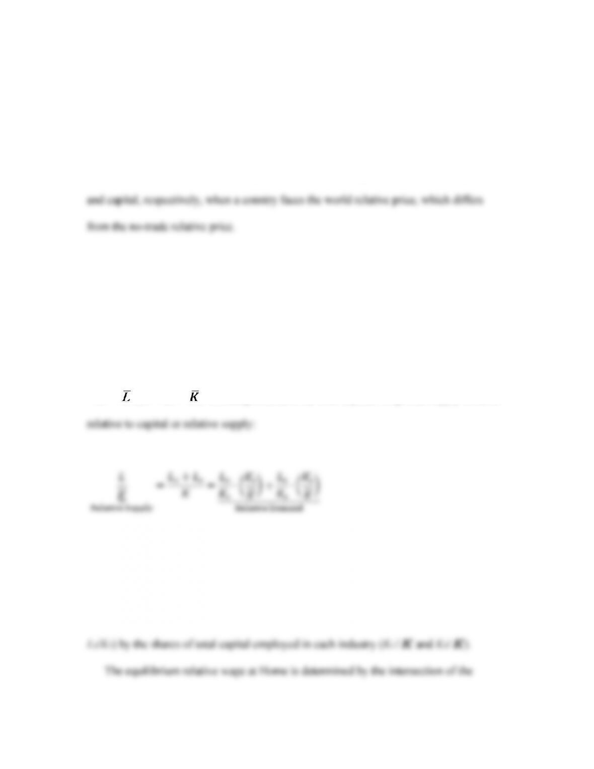
Economy-Wide Relative Demand for Labor Recall that the total amount of labor
(capital) in an economy is equal to the sum of the labor (capital) in each industry, i.e., LC
+ LS = (KC + KS + ). Dividing total labor by total capital, we get the supply of labor
The relative demand or demand for labor relative to capital, shown on the right-hand
side, is a weighted average of the labor–capital ratio in each industry. The weighted
average is calculated by multiplying the labor–capital ratio for each industry (LC/KC and
Increase in the Relative Price of Computers Because of free trade, Home faces a
higher relative price of computers, which drives it to further specialize in the production
of computers, shifting away resources from the production of shoes. The increase in the
With production specializing in computers, the fall in the relative demand for labor in
the shoe industry causes a decrease in the relative wage from (W/R)1 to (W/R)2. The lower
relative wage, in turn, induces an increase in the number of workers hired per unit of
capital in each industry, shown by the movement along the relative demand curves for
Determination of the Real Wage and Real Rental
Change in the Real Rental The rental on capital in computers (shoes) is equal to its
marginal product multiplied by the price of computers (shoes):
R = PC • MPKC and R = PS • MPKS
Because the labor–capital ratio increases in both industries due to the higher world
capital–intensive).
Change in the Real Wage Similarly, the wage in computers (shoes) is equal to its
marginal product multiplied by the price of computers (shoes):
MPLC = W/PC ↓ and MPLS = W/PS ↓
where we see that labor experiences a decrease in real wage in terms of the quantity of
experiences a fall in real terms in rental on capital and a rise in real terms in wage. This
means that labor in Foreign is better off with free trade and the capital owner is worse off.
This finding is summarized by the following Stolper–Samuelson theorem.
Stolpe–Samuelson Theorem In the long run, when all factors are mobile, an increase in
Changes in the Real Wage and Rental: A Numerical Example
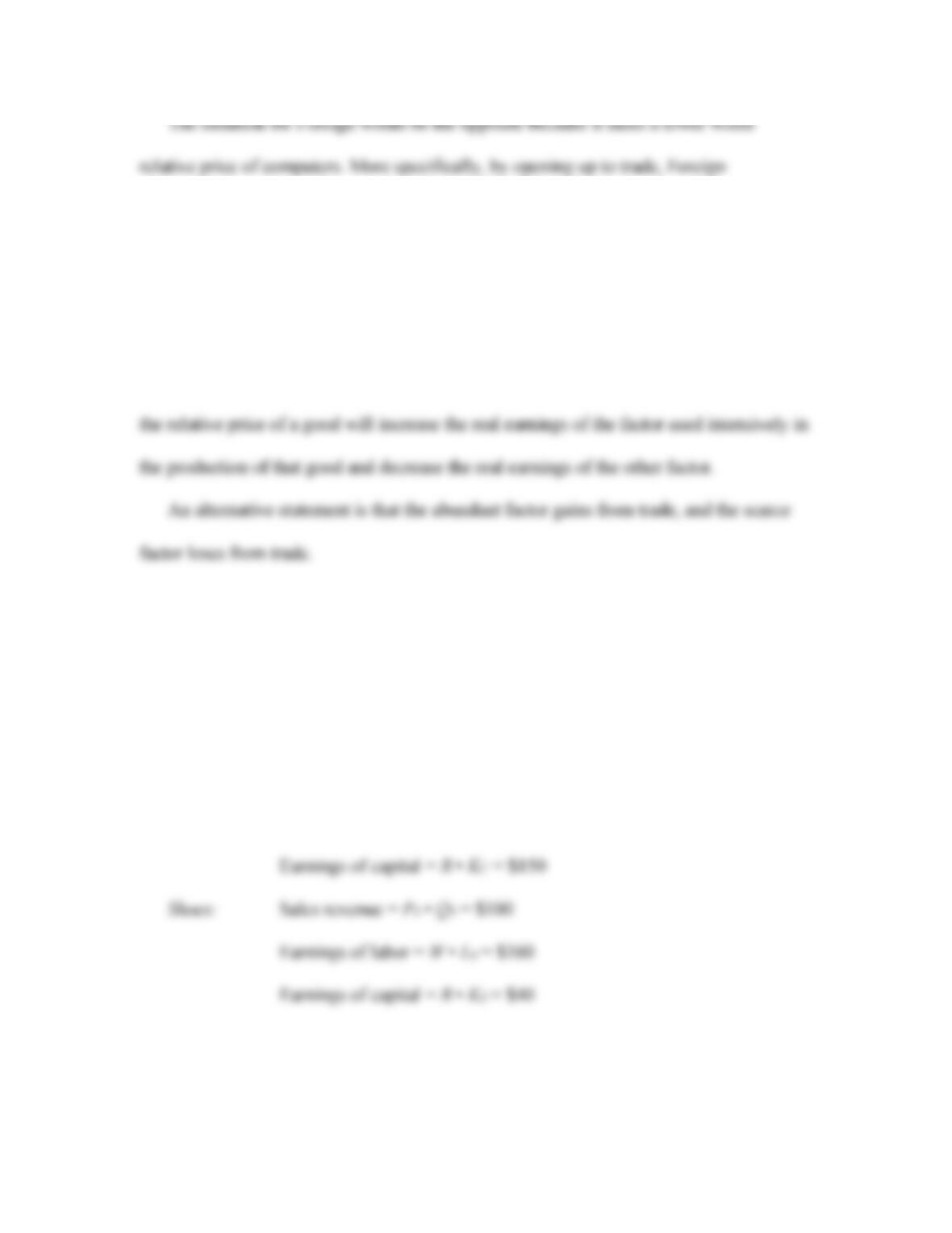
Suppose the following:
Computers: Sales revenue = PC • QC = $100
Earnings of labor = W • LC = $50
Note that shoes are more labor-intensive than computers because the share of total
revenue paid to labor in shoes (60/100 = 60%) is more than that share in computers
(40/100 = 40%). Under free trade, the relative price of computers rises as follows:
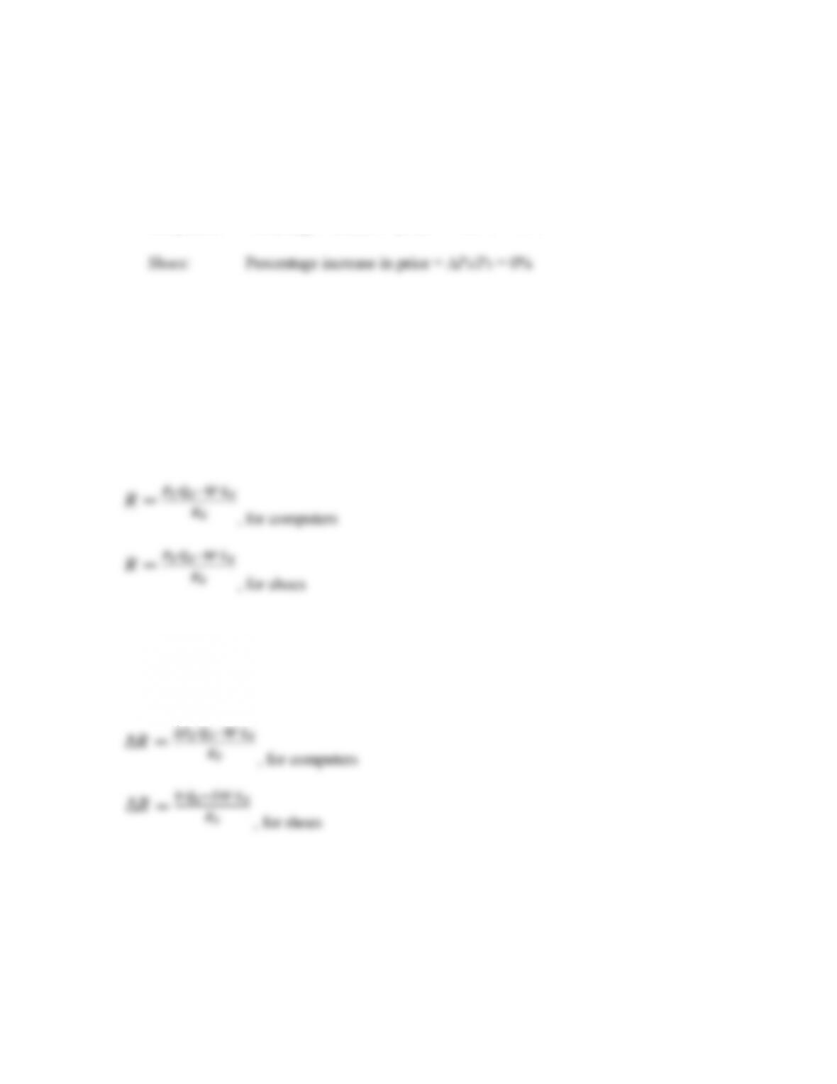
Computers: Percentage increase in price = ∆PC/PC = 10%
To determine the impact of the higher relative price of computers on the rental on
capital for each industry, we subtract the payments to labor from total sales revenue and
divide the difference by the amount of capital:
We now add in the information pertaining to the increase in the price of computers:
Rewriting the previous equations in terms of percentage changes, we have the
following:
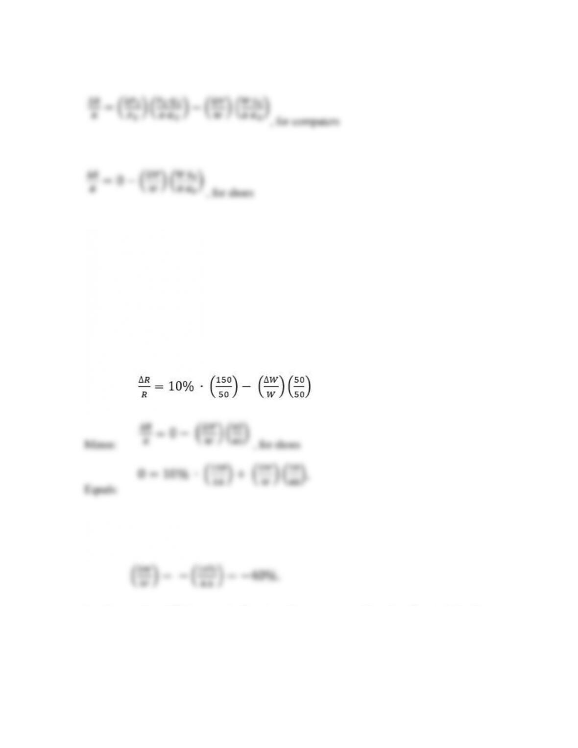
where ∆PC/PC is the percentage change in the price of computers, ∆W/W is the
percentage change in the wage, and ∆R/R is the percentage change in the rental on
capital.
Substituting the numbers given and subtracting one equation from the other, we get
, for computers
which gives the change in wages as
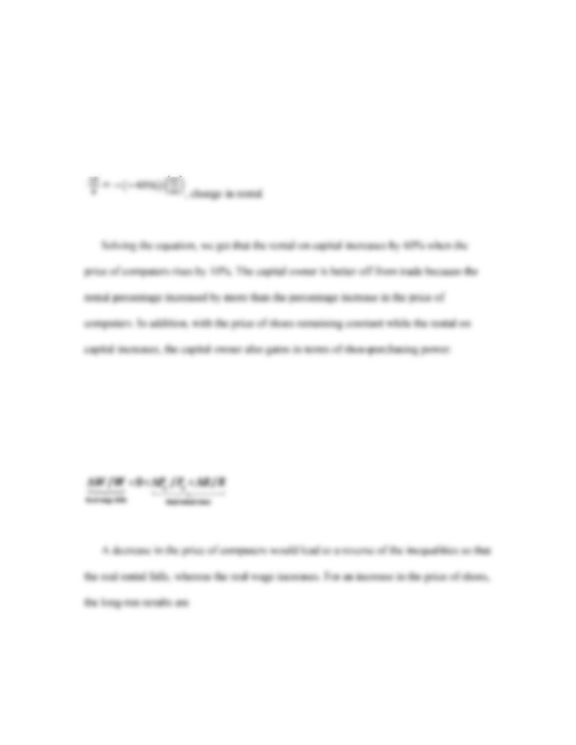
In other words, a 10% increase in the price of computers resulting from free trade leads to
a fall in the wage by 40%. This means that the real wage, measured in terms of labor
being able to purchase either computers or shoes, has fallen, so labor is worse off.
The change in the rental paid to capital (∆R/R) can be found by substituting the
percentage change in the wage (–40%) in the preceding equations for shoes or computers.
For example,
General Equation for the Long-Run Change in Factor Prices The long-run results due
to an increase in the price of computers are given by the following: