Unlock document.
This document is partially blurred.
Unlock all pages and 1 million more documents.
Get Access
18 Balance of Payments II: Output, Exchange Rates, and
Macroeconomic Policies in the Short Run
Notes to Instructor
Chapter Summary
This chapter develops a standard short-run macroeconomic model for the open economy.
It begins with an overview of the components of demand and their determinants, then
derives a goods market equilibrium using the Keynesian cross. The next two sections
Comments
This chapter is very dense because it combines material that would easily take several
weeks to cover in an intermediate macroeconomics course. For those classes in which
intermediate macroeconomic theory is a prerequisite, this material can be taught
relatively quickly, emphasizing the richer role of the trade balance in equilibrium
outcomes. For these students, Sections 1 through 4 probably can be condensed, treating
1. Demand in the Open Economy
a. Preliminaries and Assumptions
b. Consumption
i. Marginal Effects
c. Investment
d. The Government
e. The Trade Balance
f. Exogenous Changes in Demand
i. Side Bar: Barriers to Expenditure Switching: Pass-Through and the J
Curve
2. Goods Market Equilibrium: The Keynesian Cross
a. Supply and Demand
3. Goods and Forex Market Equilibria: Deriving the IS Curve
a. Equilibrium in Two Markets
4. Money Market Equilibrium: Deriving the LM Curve
a. Money Market Recap
5. The Short-Run IS‒LM‒FX Model of an Open Economy
a. Macroeconomic Policies in the Short Run
6. Stabilization Policy
a. Application: The Right Time for Austerity
b. Problems in Policy Design and Implementation
i. Policy Constraints
ii. Incomplete Information and the Inside Lag
c. Application: Macroeconomic Policies in the Liquidity Trap
7. Conclusions
Lecture Notes
This chapter connects exchange rate movements to the national economy using the IS‒
LM model. By combining the theories of exchange rate determination with the balance of
payments accounting, we can better understand how exchange rate movements affect key
1 Demand in the Open Economy
In previous chapters, we took the level of output as a given, allowing us to abstract from
fluctuations in the goods market. This assumption is acceptable for long-run economic
analysis because the level of output is determined by the factors of production. In the
Preliminaries and Assumptions
■ Home and foreign price levels, and , are constant so expected inflation is
■ GDP is taken as equivalent to GNDI.
Consumption
Consumption, C, is a function of disposable income, Yd = Y − :
Marginal Effects The slope of the consumption function is the marginal propensity to
Investment
Firms engage in capital investment projects only when the real return on the project
exceeds the cost of borrowing. The firm’s borrowing cost is the expected real interest
This relationship is illustrated in the investment function, Figure 18-2.
The Government
The government collects taxes, T, from households and spends government
The government’s tax revenue may not exactly equal its government consumption
spending.
■ G > T: Budget deficit
Fiscal policy refers to decisions about taxes and government consumption. Based on our
assumptions, these values are taken as given:
The Trade Balance
The quantities of exports and imports, and therefore the trade balance, are all directly
affected by exchange rates. We need to study the variables that influence the trade
balance so we can make it endogenous. Those variables include the real exchange rate,
the level of home income, and the level of foreign income.
The Role of the Real Exchange Rate The change in spending patterns in response to
exchange rate fluctuations is known as expenditure switching (between foreign and
home purchases).
Recall that the real exchange rate is defined as
We can use this expression to understand how expenditure switching works:
■ ↑ q → real depreciation of the home currency ‒ foreign goods are relatively more
■ ↓ q → real appreciation of the home currency ‒ home goods are relatively more
The Role of Income Levels When income rises, people generally buy more of
everything, including imports. But we need to realize that our exports are other countries’
imports. And, of course, our imports are their exports. That means an increase in home
income increases home imports and foreign exports. Similarly, an increase in foreign
income increases foreign imports and home exports.
The home country’s income also affects the trade balance:
Finally, the foreign country’s income affects the trade balance:
■ ↑ Y* → foreign country increases spending on all goods → home country exports
In summary, the trade balance is a function of three variables:
The trade balance is illustrated as a function of the real exchange rate shown in Figure
H E A D L I N E S
The Curry Trade
In 2009, the British pound weakened dramatically vis-à-vis the euro. That led to some
interesting changes in trade across the English Channel.
Discussion Questions:
■ Shipping French food products to the United Kingdom, then shipping them back
to France is costly. Given these high transportation costs, explain how it is
possible for customers in France to buy those products from the United Kingdom
moved after 2009.
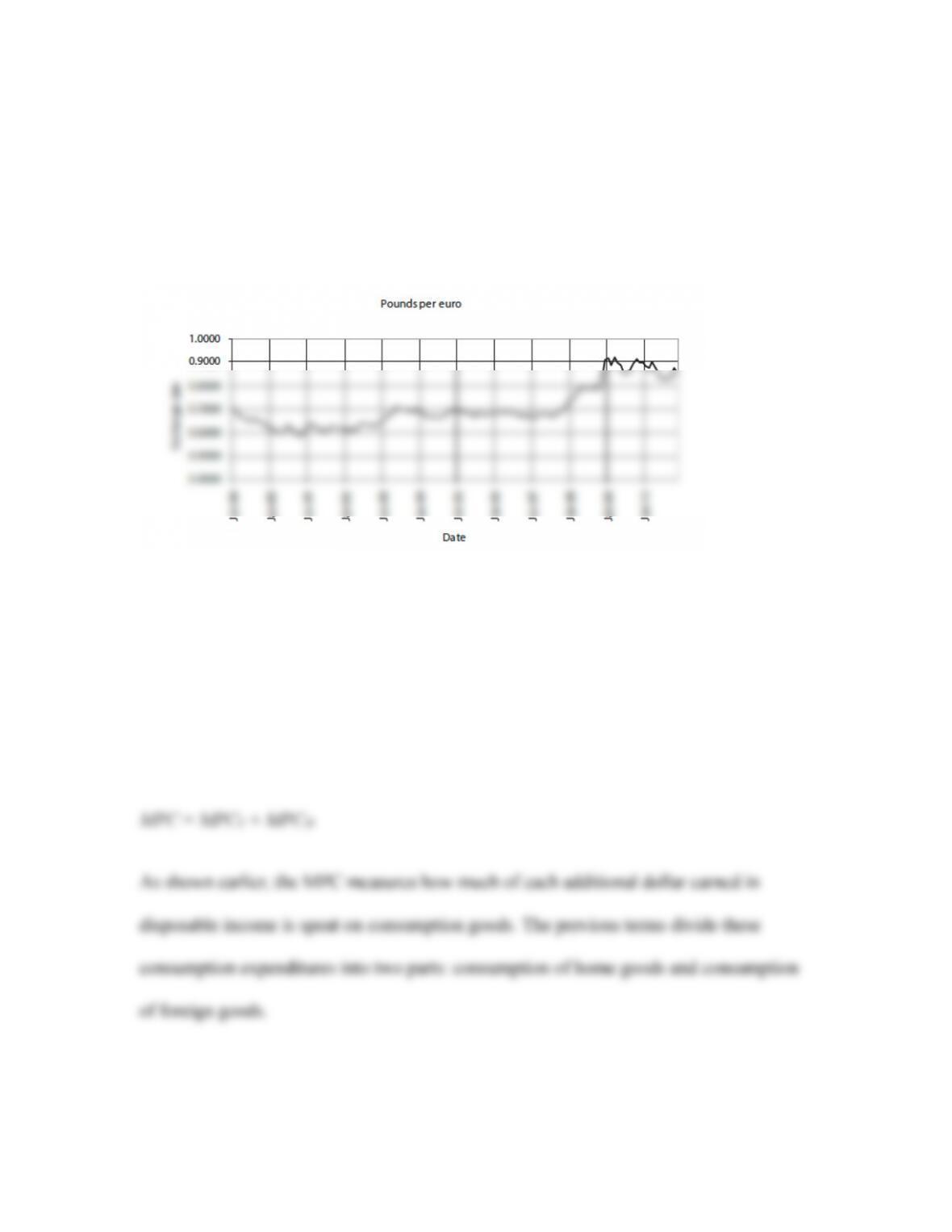
Here’s a graph of the pound‒euro exchange rate from 1999 through November 2010.
The effect of a change in output on the trade balance can be thought of in terms of the
marginal propensity to consume. Let MPCF denote the marginal propensity to consume
foreign imports and MPCH denote the marginal propensity to consume home goods and
services:
APPLICATION
The Trade Balance and the Real Exchange Rate
Figure 18-4 reports the real effective exchange rate relative to the trade balance in the
United States, 1975 to 2006. The real effective exchange rate measures real depreciation
and appreciation in the United States relative to a basket of other countries (weighted by
how much the United States trades with each country). This provides a comprehensive
Exogenous Changes in Demand
This section considers the sources of exogenous shocks to demand:
■ An exogenous change in consumption shifts the consumption function. Panel (a)
of Figure 18-6 shows an exogenous increase in consumption. When there is an
exogenous increase in consumption, the consumption function shifts up. For any
■ An exogenous change in investment shifts the investment function. Figure 18-6,
panel (b), shows an exogenous increase in investment. An exogenous increase in
investment shifts the investment function to the right. For any given interest rate,
■ An exogenous change in the trade balance shifts the trade balance function. Panel
(c) of Figure 18-6 shows an exogenous increase in the trade balance. An
exogenous increase in the trade balance shifts the trade balance function up. For
any given real exchange rate, the trade balance is higher. An exogenous decrease
S I D E B A R
Barriers to Expenditure Switching: Pass-Through and the J Curve
There are two key mechanisms at work when the real exchange rate changes.
■ A nominal depreciation is associated with a real depreciation (because prices are
fixed).
Trade Dollarization, Distribution, and Pass-Through
We assumed that all prices are set in local currency and that these prices are fixed in the
short run. In reality, some home goods may be priced in foreign currency. To understand
how this affects trade, define these two pricing schemes (treating the United States as the
foreign country):
Therefore, we can define the price of foreign goods relative to dollar-priced home goods
and relative to local-currency-priced home goods:
Based on the previous weighting, we can derive the price of goods sold in the home
country relative to those sold in the foreign country (e.g., the real exchange rate):
exchange rates are passed through to real exchange rates. In the model given in the text,
we assume d = 0.
Table 18-1 reports the shares of exports and imports denominated in U.S. dollars and
euros (roughly equivalent to the share d previously). Note that if a large share of the trade
balance is denominated in U.S. dollars, then a depreciation or appreciation of the U.S.
The J Curve
A real depreciation improves a country’s trade balance through boosting exports and
reducing imports. In reality, this process takes time because orders for exports and
imports are placed in advance and the payment occurs much later, at the time of delivery.
It may take time for firms and intermediaries to fully adjust their orders.
Although exports continue to sell, for a time, in the same quantity at the same
domestic price, the domestic price paid for imports will increase (depending on the
degree of pass-through). Thus, the quantity of imports into the country stays the same,
but these goods cost more, increasing total spending on imports. The overall effect is a
decrease in the trade balance. Therefore, before firms adjust their orders, the total
spending on imports rises and total spending on exports remains the same, so the trade
2 Goods Market Equilibrium: The Keynesian Cross
This section uses the traditional Keynesian cross approach to goods market equilibrium.
Supply and Demand
The total aggregate supply of final goods and services is equal to total output, GDP − Y:
We know that the national income accounting identity says the supply of output is equal
to the demand for final goods and services. The demand for goods and services is given
by the previous components:
In equilibrium, demand (D) must equal aggregate output (Y). Substituting Y
for D in the equation for aggregate demand, we obtain the goods market equilibrium
condition:
Determinants of Demand
The factors that can affect demand include
■ The home nominal interest rate (i)
We begin by analyzing the impact of a change in home output. Suppose Y rises by $1.
Consumption spending will rise by +$MPC. And imports will rise by +$MPCF. The trade
balance will change by −$MPCF. The net change in aggregate demand will be $(MPC −
(which, in this case, includes spending on both domestic and foreign goods).
So far our graph includes only aggregate demand:
When demand is graphed against output (income, Y), the slope of the line will be less
than 1.0. This graph shows how demand changes as Y changes. What is the one point at
which spending equals output?
To answer that question, we need another line in our graph, the line showing all
possible points of equilibrium. The equation of that line is D = Y. By a coincidence of
To see why the goods market adjusts to equilibrium, consider the following cases. Let
Y1 denote the equilibrium (point 1 in Figure 18-7).
Factors That Shift the Demand Curve
In the following examples, the first example is illustrated in panel (b) of Figure 18-6 (as
an increase in demand).
■ Government purchases:
↑ ⇒ D shifts upward ⇒ ↑ Y
■ Interest rate: i
↓ i ⇒ ↑ l(i) ⇒ D shifts upward ⇒ ↑ Y
■ Nominal exchange rate: E
↑ E ⇒ ↑ TB(/ , Y − T, Y* − T*) ⇒ D shifts upward ⇒ ↑ Y
Summary
The Keynesian cross is derived from the relationship between the demand for goods and
services, which depends on income, and their supply, or output, Y. Changes in demand
not associated with changes in output (Y) lead to a shift in the demand curve for goods
and services.
3 Goods and Forex Market Equilibria: Deriving the IS Curve
To derive the economy’s general equilibrium, we must consider the equilibrium in three
markets: the goods market, the money market, and the forex market. Students probably
will be familiar with the concept of general equilibrium (even if this term was not
Equilibrium in Two Markets
In the IS‒LM diagram, we study equilibrium in three markets: the goods market, the
forex market (IS), and the money market (LM). This section focuses on the IS curve.
The IS curve shows combinations of output Y and interest rate i in which the goods
and the forex markets are in equilibrium.
The IS curve is plotted with interest rate i on the vertical axis and output Y on the
Forex Market Recap
The forex market equilibrium is given by the uncovered interest parity (UIP) condition:
The return on domestic deposits, the nominal interest rate i, must equal the expected
market equilibrium, we obtain the equilibrium interest rate i and nominal exchange rate
E.
Deriving the IS Curve
This section derives the shape of the IS curve through examining changes in the interest
rate.
Initial Equilibrium Using the diagrams, the equilibrium output and interest rate are
given from the goods market and forex market:
■ Goods market: The level of output from the goods market equilibrium must be a
It may be worthwhile to point out that lining up the diagrams correctly helps students
avoid mistakes because they can check for consistency across the two (eventually, three)
markets.
A Fall in the Interest Rate To derive the IS curve, consider how a change in the interest
rate affects the demand for goods and the forex market. Figure 18-8 illustrates how a
decrease in the interest affects the two markets:
■ Panel (a): ↓ i ⇒ ↑ I(i) ⇒ D shifts upward ⇒ ↑ Y
Note that expenditure switching is a source of demand for goods and services not
present in the closed economy. In the open economy, lower interest rates increase


