Factors That Shift the IS Curve
The following exogenous factors lead to a shift in the IS curve. For each bullet, the first
example is an increase in demand, as illustrated in Figure 18–9.
■ Government purchases:
■ Taxes:
↓ ⇒ ↑ C(Y − ) ⇒ D shifts up ⇒ ↑ Y
■ Foreign interest rate or expected future exchange rate: i* or Ee
■ Home or foreign price level: or
These changes can be summarized by expressing the IS curve as a function:
Summing Up the IS Curve
The IS curve is downward-sloping because a decrease in the interest rate leads to an
increase in investment demand and the trade balance, which increases the demand for
goods and therefore output in the short run.
4 Money Market Equilibrium: Deriving the LM Curve
The money and assets market was modeled in earlier chapters. The LM curve is based on
that model. The LM curve shows combinations of output and the nominal interest rate
that bring the money market into equilibrium.
Money Market Recap
We continue to work with the short-run model in which the price level is fixed.
Therefore, the nominal interest rate adjusts to bring the money market into equilibrium.
The money market equilibrium is the point at which real money demand equals real
money supply:
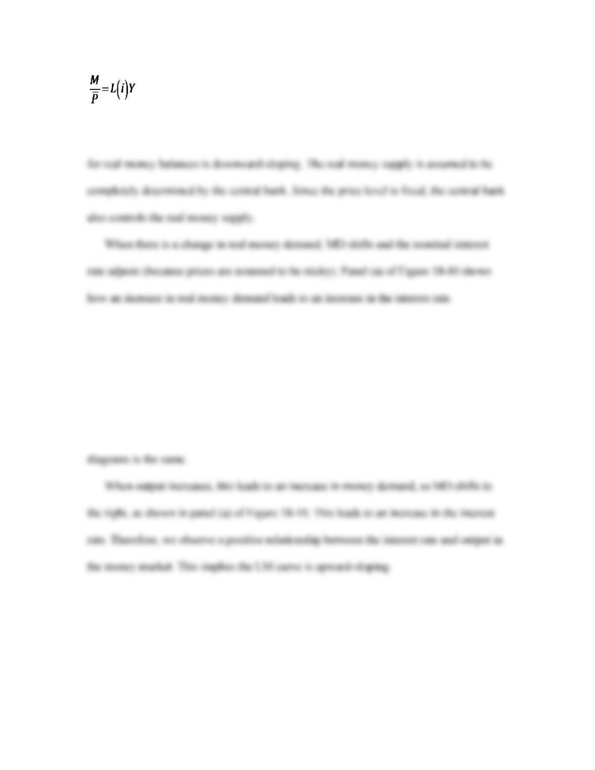
Real money demand (MD) varies inversely with the nominal interest rate, so the demand
Deriving the LM Curve
Figure 18-10 illustrates how we can use the money market to derive the LM curve. Note
that the money market and the LM diagram share a vertical axis (the interest rate), so
they can be aligned horizontally. In this way, we ensure that the interest rate in both
Factors That Shift the LM Curve
We focus most of our attention on the real money supply. A change in the real money
supply is the main exogenous variable that shifts the LM curve. Figure 18-11 shows how
an increase in real money supply leads to a rightward shift in the LM curve.
Real money supply: M/
These changes can be summarized through expressing the LM curve as a function:
In general, any shock that increases interest rates for a given level of output (e. g., a given
L) will shift the LM curve to the left; any shock that decreases interest rates will shift the
LM curve to the right.
Exogenous changes in money demand will also shift the LM curve. These changes
Summing Up the LM Curve
The LM curve is upward–sloping because an increase in output leads to an increase in
real money demand, which increases the nominal interest rate in the short run. Similarly,
a decrease in output reduces real money demand and the nominal interest rate.
5 The Short–Run IS‒LM‒FX Model of an Open Economy
We can now combine the IS‒LM diagram with the FX market diagram to study how
Macroeconomic Policies in the Short Run
We focus on two main policy actions:
■ Monetary policy is any change in the nominal money supply implemented by the
The effects of these policies depend critically on the nation’s exchange rate regime.
Assumptions:
■ The economy is initially at long-run equilibrium (full employment, expected
inflation equals actual inflation).
Temporary Policies, Unchanged Expectations Remember that to examine temporary
shocks to the economy, we assume investors do not change exchange rate expectations.
We make this assumption to study how temporary policies (designed to affect output in
the short run) affect the economy.
Monetary Policy Under Floating Exchange Rates
■ Monetary expansion (shown in Figure 18-13):
■ Direct effect:
■ Indirect effects:
↑ Y ⇒ ↑ C
Note that a monetary expansion leads to an exchange rate depreciation and a decrease
in the interest rate: both of these imply an increase output.
■ Monetary contraction: LM shifts left ⇒ DR shifts up. Effects: ↑ i, ↓ Y, ↓ E ⇒ ↓ I,
↓ C ↓ TB.
■ Comparison with the closed economy: In the closed economy, there would be no
expenditure switching, so the effects of monetary policy on output would be
weakened.
Monetary Policy Under Fixed Exchange Rates
Monetary expansion (shown in Figure 18-14):
Note that if the country is committed to a fixed exchange rate regime, the central bank
cannot change the real money supply. Changing the real money supply affects the
Fiscal Policy Under Floating Exchange Rates
■ Fiscal expansion (increase in G; shown in Figure 18-15):
■ Direct effect:
■ Indirect effects:
↑ i ⇒ ↓ I
Note that an increase in government spending (or a decrease in taxes) leads to an
increase in output. However, the increase in output that comes from the increase in
■ Fiscal contraction (decrease in G): IS shifts left ⇒ DR shifts down.
■ Comparison with the closed economy: In the closed economy, there would be no
Note that we can also study fiscal policy in terms of taxes.
■ Fiscal expansion (tax cut): ↓ T ⇒ ↑ C ⇒ ↑ IS shifts right ⇒ DR shifts up.
■ Fiscal contraction (tax increase): ↑ T ⇒ ↓ C: IS shifts left ⇒ DR shifts down.
Fiscal Policy Under Fixed Exchange Rates
It is important to note that under a fixed exchange rate regime, the real money supply
must be adjusted to ensure the nominal exchange rate remains fixed. This means that any
fiscal policy action will be paired with a change in the money supply.
■ Fiscal expansion (increase in G; shown in Figure 18-16):
■ Direct effects:
↑ G ⇒ ↑ Y
■ Indirect effects:
E no change
■ Note that in this case, monetary policy amplifies the effects of fiscal policy
through eliminating crowding out (because interest rates must remain unchanged
■ Fiscal contraction (decrease in G):
↓ G ⇒ ↓ D ⇒ IS shifts left ⇒ DR shifts down
Summary
The effects of monetary and fiscal expansion in floating and fixed exchange rate regimes
are summarized in the table. We can see that it is not possible to have autonomous
monetary policy in a fixed exchange rate regime. However, autonomous fiscal policy is
possible in a fixed exchange rate regime.
6 Stabilization Policy
Stabilization policy refers to monetary and fiscal policies designed to keep output at or
near full employment level. If the economy experiences an adverse shock, fiscal policy
can increase demand through shifting the IS curve to the right, or monetary policy can
Problems in Policy Design and Implementation
Although the model provides policy makers with a relatively straightforward way to
respond to shocks, in practice, their ability to implement such policies is limited by
several factors.
Policy Constraints Policy makers may not have the freedom to implement stabilization
policies. For example, fixed exchange rates or other “rules” for policy may limit their
Incomplete Information and the Inside Lag The model assumes that policy makers can
observe the state of the economy in real time. In practice, they observe macroeconomic
data with a lag. The lag between the timing of the shock and the policy action is known
as an inside lag. In addition, institutional factors severely limit the timely implementation
of fiscal policy.
Policy Response and the Outside Lag Even with perfect information on the economy, it
may take time for an implemented policy to have real economic effects. This is known as
an outside lag. The outside lag is a particular problem for monetary policy. While the
Long–Horizon Plans If households and businesses making decisions about consumption
and investment plan over long horizons, they may be less responsive to policy changes.
For example, if a business borrows to finance capital expansion, it will likely borrow over
Weak Links from the Nominal Exchange Rate to the Real Exchange Rate The model
assumes that changes in nominal exchange rates translate into changes in the real
exchange rate, the rate that matters for export/import decisions. In practice, there is
Pegged Currency Blocs Some countries use a combination of fixed and floating
exchange rates to limit one country from boosting export demand through a real effective
Weak Links from the Real Exchange Rate to the Trade Balance The model assumes
that changes in the real exchange rate imply changes in the trade balance. In practice, the
link between the two may be weak because of transactions costs. The existence of these
APPLICATION
Macroeconomic Policies in the Liquidity Trap
The financial crisis and recession of 2008–2009 provided yet another lesson in the
limitations of monetary policy. The IS curve for most developed economies shifted very
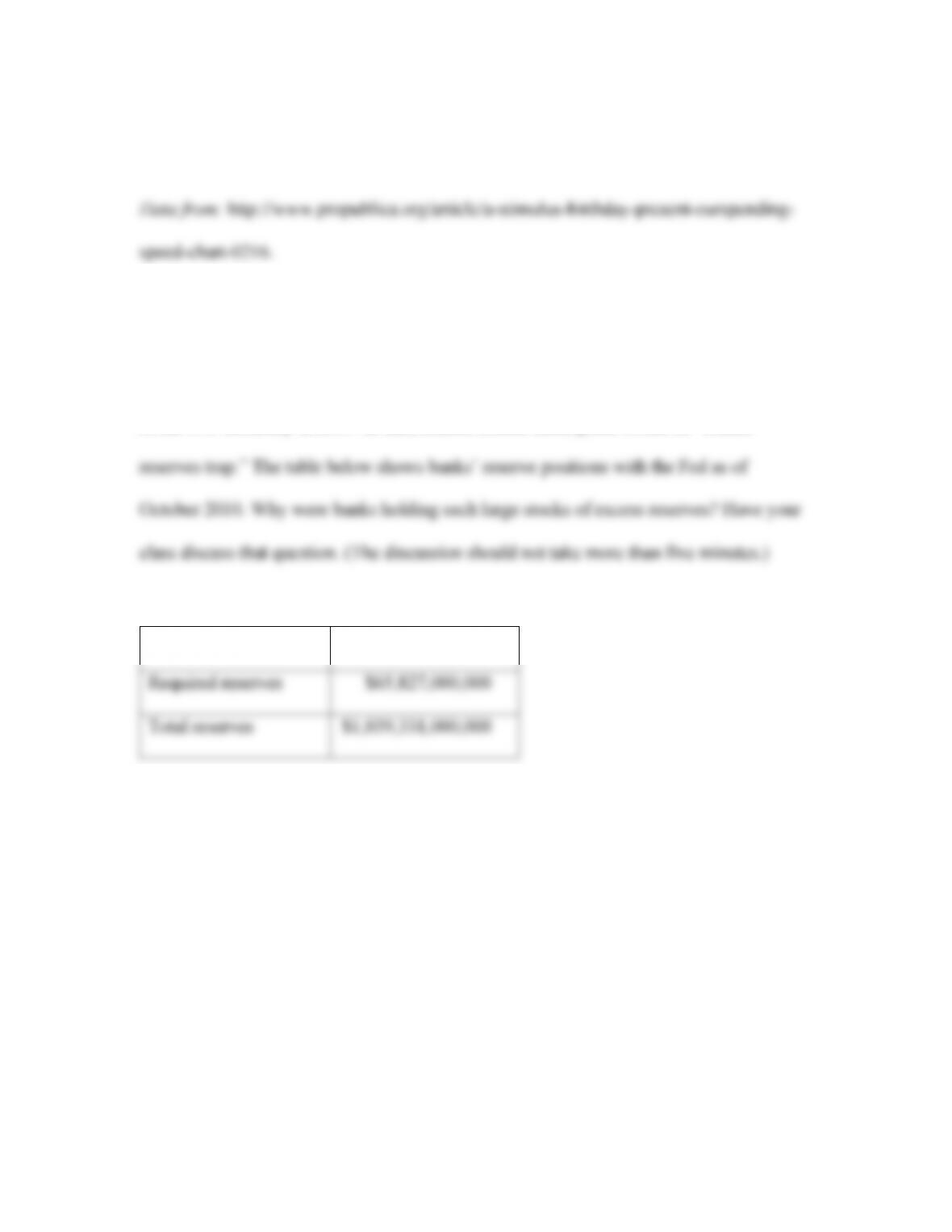
far to the left. This was caused by the extreme risk aversion of banks around the world,
positions as of October 2010:
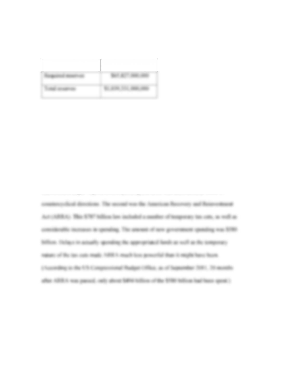
Excess reserves
$973,504,000,000
Required reserves
$65,827,000,000
Total reserves
$1,039,331,000,000
No matter how you measure it, the LM curve was effectively identical to the
horizontal axis of the IS‒LM diagram. This is the zero lower bound (ZLB) problem.
Under this situation, fiscal policy is the only tool that can be used to stimulate the
economy. Because monetary policy is ultra-accommodating, the fiscal policy multiplier
will be large.
The fiscal stimulus in the United States took two forms. First were the automatic
stabilizers, changes in government spending and taxes that automatically move in
And, of course, temporary tax cuts never have the multiplier impact of permanent tax
cuts. We don’t need to look any further than the permanent income model of consumption
to verify that fact.
7 Conclusions
This chapter builds a short-run macroeconomic model for the open economy. The trade
balance implies an additional source of demand for goods and services. Changes in
relative prices and nominal exchange rates allow for expenditure switching between
countries.
The effects of monetary and fiscal policy are quite different under different exchange
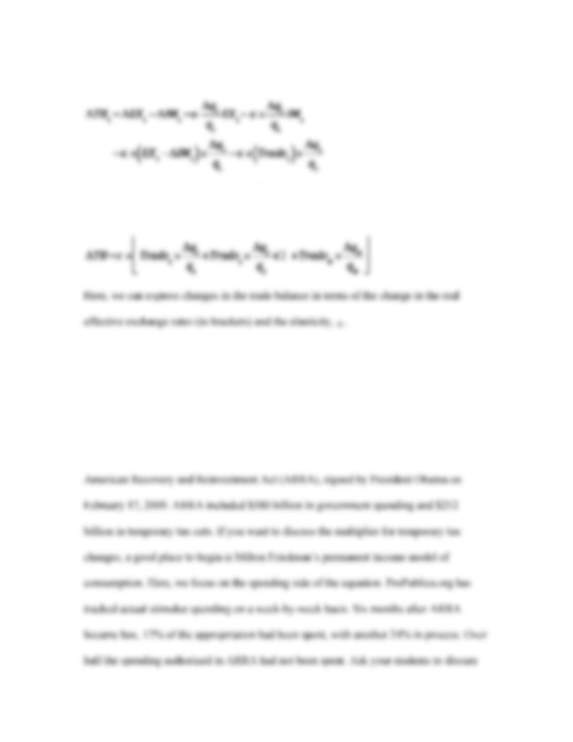
Appendix 1: The Marshall‒Lerner Condition
This appendix considers the assumption that a depreciation leads to an increase in the
trade balance. For simplicity, assume TB = 0; therefore, EX = IM.
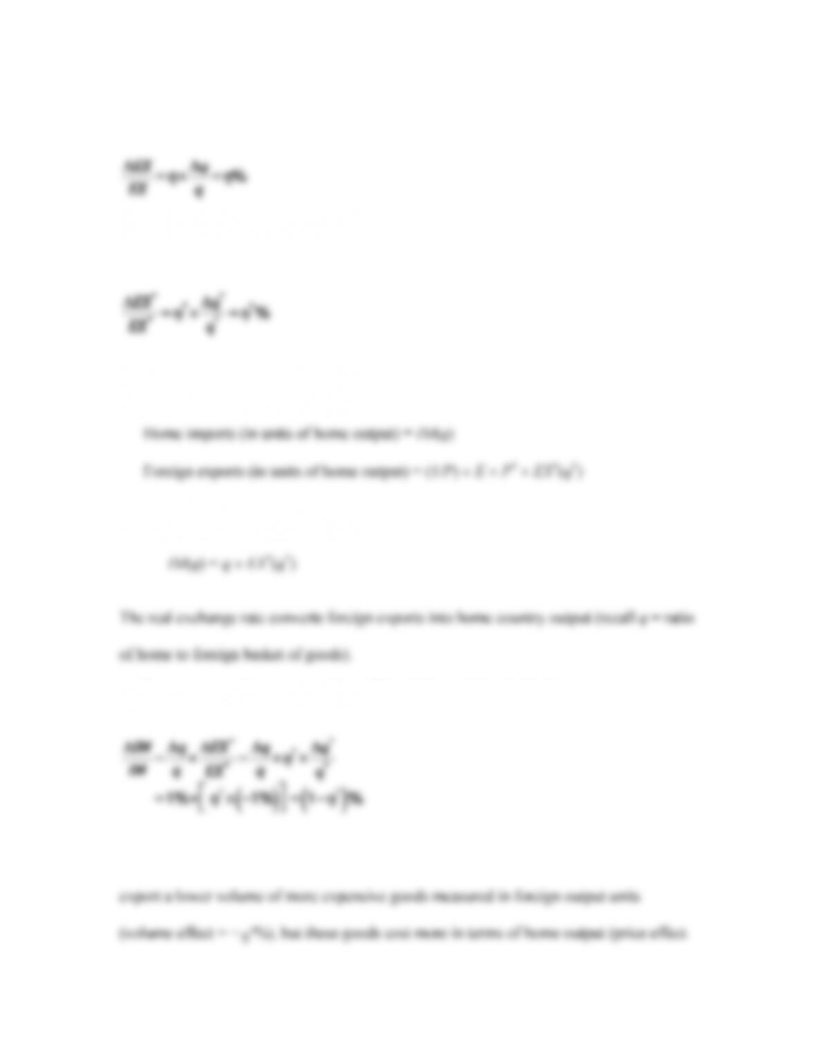
η
:
For the foreign country:
Note that EX* = IM, from the home country’s perspective.
These expressions must be equal:
In percentage changes, assuming a 1% real depreciation in the home country:
From the previous expression, we see there are two effects of a depreciation. Foreigners
η
Following a change in the real exchange rate, exports change by
η
%, imports change
by (1 −
η
*)%. In the case of a real depreciation, the trade balance increases only if
η
> 1
η
η
This expression is known as the Marshall‒Lerner condition. The trade balance will
increase following a depreciation only if trade volume changes are sufficiently large (e.g.,
they are sufficiently elastic) to offset the price effects.
This helps us explain the J-curve effect. In this case, volumes are relatively
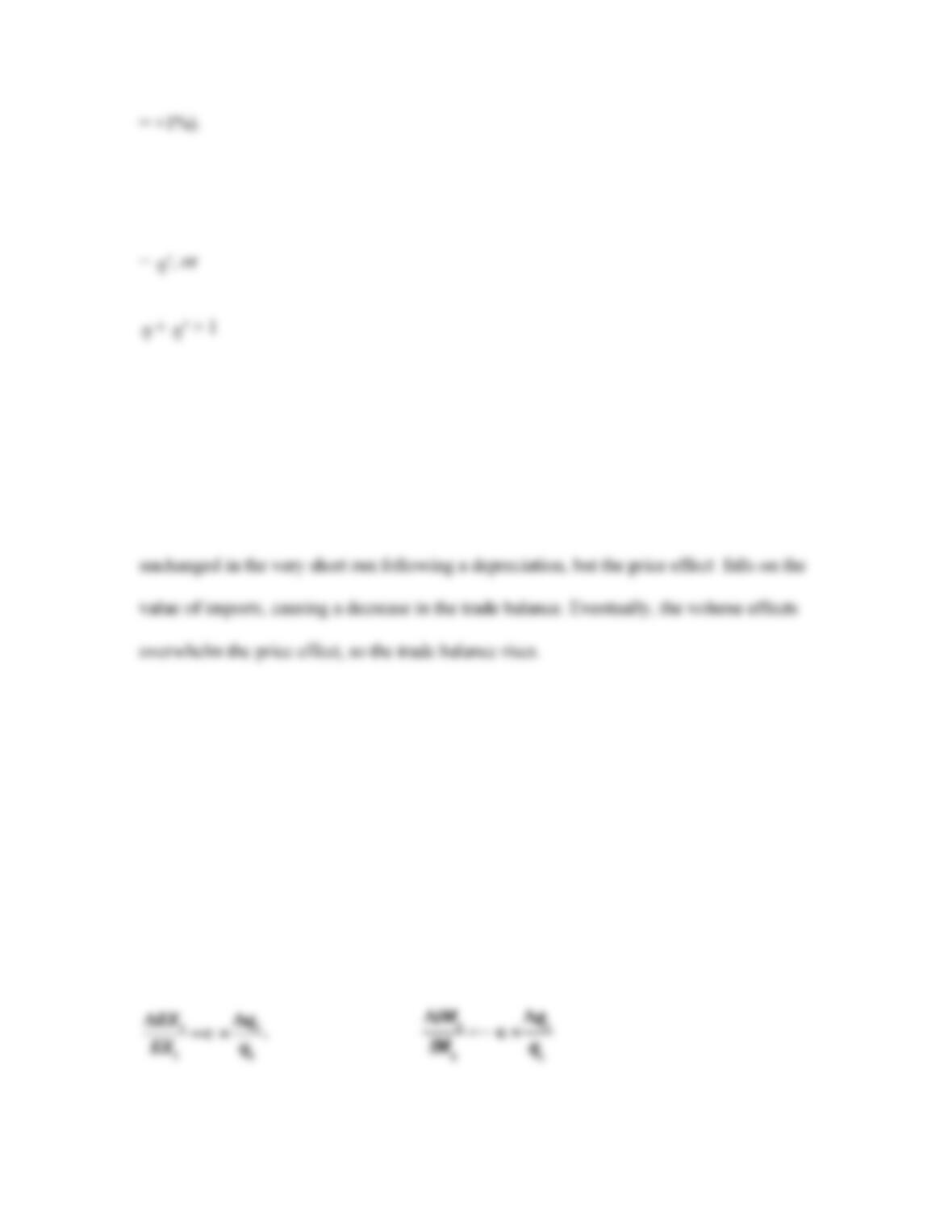
Appendix 2: Multilateral Real Exchange Rates
This appendix extends the model to more than two countries. Here, we assume there are
N countries in the world. We can then examine macroeconomic consequences in terms of
the real effective exchange rates.
Consider the effects of a small change in the exchange rate. For country 1, the
changes in exports and imports are expressed as
where ∈ > 0 is an elasticity. The change in the trade balance is therefore
Note that this expression holds for each individual country. Adding up the change in the
trade balances for each individual country gives us
Teaching Tips
Teaching Tip 1: (This is related to the Application: Macroeconomic Policies in the
Liquidity Trap.) As the application notes, once monetary policy reaches the zero lower
bound, it is up to fiscal policy to stimulate the economy. The fiscal stimulus was the
the impact of this lag (which we might call the bureaucratic lag) on the economic
recovery.
Teaching Tip 2: (Also related to the Application: Macroeconomic Policies in the
Liquidity Trap.) The textbook uses Keynes’s term “liquidity trap” to describe the state
of the U.S. economy in 2009. In fact, a more correct description would be “excess
Excess reserves
$973,504,000,000
Required reserves
$65,827,000,000
Total reserves
$1,039,331,000,000
Data from: Federal Reserve System H.3 report, available for download at
http://federalreserve.gov/datadownload/Choose.aspx?rel=H.3.
IN–CLASS PROBLEMS
1. This question will compare the policies of the federal government and the Federal
Reserve and their likely effects on interest rates, exchange rates, output, and the trade
balance during the mid– to late 1970s.
a. President Lyndon Johnson and Congress passed large increases in government
spending to finance Great Society programs and the Vietnam War. Explain briefly
how such spending affects the trade balance.
Answer: A fiscal expansion leads to an increase in interest rates and an
b. Beginning in the mid-1970s, Federal Reserve Chairman Arthur Burns sought to
lower unemployment below its full employment level by decreasing interest rates.
Does this require a monetary expansion or contraction?
c. Illustrate the effects of the fiscal and monetary policies mentioned previously
using the IS‒LM‒FX market diagram. [Note the change in interest rates observed
in (b).]
Answer: See the following diagram. Because interest rates fell in the mid-1970s,
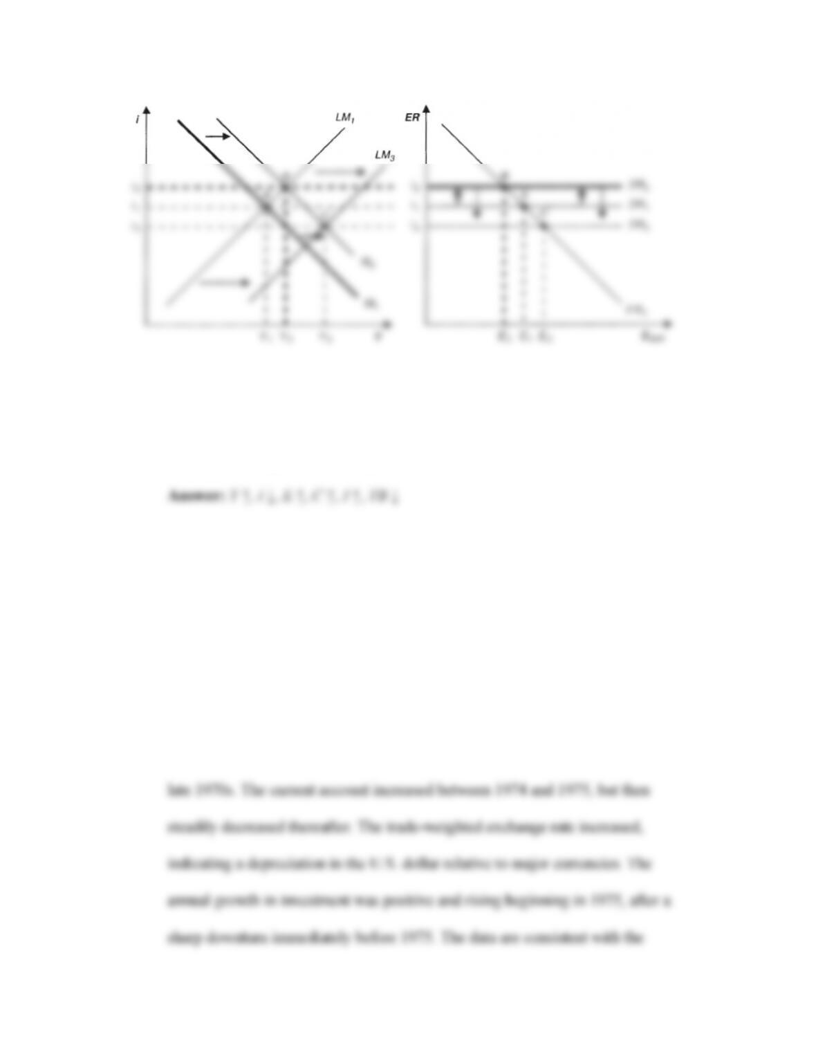
d. State the effects of these policies on the following variables: output, interest rate,
nominal exchange rate, consumption, investment, and the trade balance.
e. Go to the Federal Reserve Economics Database (FRED). Here, you can look at
graphs of the following variables (1975–78): effective federal funds rate (interest
rate), the effective exchange rate (against major currencies), current account, and
gross private investment (% change from one year ago). Based on these figures,
are the data consistent with the model in this case? Which variables, if any, do not
behave according to the model during this period?
Answer: The effective federal funds rate declined, then gradually increased in the