
Chapter 17 (6)
Output and the Exchange Rate
in the Short Run
◼ Chapter Organization
Determinants of Aggregate Demand in an Open Economy
Determinants of Consumption Demand
Determinants of the Current Account
How Real Exchange Rate Changes Affect the Current Account
How Disposable Income Changes Affect the Current Account
The Equation of Aggregate Demand
The Real Exchange Rate and Aggregate Demand
Real Income and Aggregate Demand
How Output Is Determined in the Short Run
Output Market Equilibrium in the Short Run: The DD Schedule
Output, the Exchange Rate, and Output Market Equilibrium
Deriving the DD Schedule
Factors that Shift the DD Schedule
Asset Market Equilibrium in the Short Run: The AA Schedule
Output, the Exchange Rate, and Asset Market Equilibrium
Deriving the AA Schedule
Factors that Shift the AA Schedule
Short-Run Equilibrium for the Economy: Putting the DD and AA Schedules Together
Temporary Changes in Monetary and Fiscal Policy
Monetary Policy
Fiscal Policy
Policies to Maintain Full Employment
Inflation Bias and Other Problems of Policy Formulation
Permanent Shifts in Monetary and Fiscal Policy
A Permanent Increase in the Money Supply
Adjustment to a Permanent Increase in the Money Supply
A Permanent Fiscal Expansion

98 Krugman/Obstfeld/Melitz • International Economics: Theory & Policy, Tenth Edition
Macroeconomic Policies and the Current Account
Gradual Trade Flow Adjustment and Current Account Dynamics
The J-Curve
Exchange Rate Pass-Through and Inflation
The Current Account, Wealth, and Exchange Rate Dynamics
The Liquidity Trap
Case Study: How Big Is the Government Spending Multiplier?
Summary
APPENDIX 1 TO CHAPTER 17 (6): Intertemporal Trade and Consumption Demand
APPENDIX 2 TO CHAPTER 17 (6): The Marshall-Lerner Condition and
Empirical Estimates of Trade Elasticities
Online Appendix: The IS–LM and the DD–AA Model
◼ Chapter Overview
This chapter integrates the previous analysis of exchange rate determination with a model of short-run
output determination in an open economy. The model presented is similar in spirit to the classic Mundell–
Fleming model, but the discussion goes beyond the standard presentation in its contrast of the effects of
temporary versus permanent policies. The distinction between temporary and permanent policies allows
for an analysis of dynamic paths of adjustment rather than just comparative statics. This dynamic analysis
brings in the possibility of a J-curve response of the current account to currency depreciation. The chapter
concludes with a discussion of exchange rate pass-through, that is, the response of import prices to
exchange rate movements.
The chapter begins with the development of an open-economy fixed-price model. An aggregate demand
function is derived using a Keynesian cross diagram in which the real exchange rate serves as a shift
parameter. A nominal currency depreciation increases output by stimulating exports and reducing imports,
given foreign and domestic prices, fiscal policy, and investment levels. This yields a positively sloped
output-market equilibrium (DD) schedule in exchange rate output space. A negatively sloped asset-market
equilibrium (AA) schedule completes the model. The derivation of this schedule follows from the analysis
of previous chapters. For students who have already taken intermediate macroeconomics, you may want to
point out that the intuition behind the slope of the AA curve is identical to that of the LM curve, with the
additional relationship of interest parity providing the link between the closed-economy LM curve and the
open-economy AA curve. As with the LM curve, higher income increases money demand and raises the
home-currency interest rate (given real balances). In an open economy, higher interest rates require currency
appreciation to satisfy interest parity (for a given future expected exchange rate).
The effects of temporary policies, as well as the short-run and long-run effects of permanent policies, can
be studied in the context of the DD–AA model if we identify the expected future exchange rate with the
long-run exchange rate examined in Chapters 15 (4) and 16 (5). In line with this interpretation, temporary
policies are defined to be those that leave the expected exchange rate unchanged, while permanent policies
are those that move the expected exchange rate to its new long-run level. As in the analysis in earlier
chapters, in the long run, prices change to clear markets (if necessary). Although the assumptions concerning
the expectational effects of temporary and permanent policies are unrealistic as an exact description of an
economy, they are pedagogically useful because they allow students to grasp how differing market
expectations about the duration of policies can alter their qualitative effects. Students may find the

Chapter 17 (6) Output and the Exchange Rate in the Short Run 99
distinction between temporary and permanent, on the one hand, and between short run and long run on the
other, a bit confusing at first. It is probably worthwhile to spend a few minutes discussing this topic.
Both temporary and permanent increases in money supply expand output in the short run through exchange
rate depreciation. The long-run analysis of a permanent monetary change once again shows how the well-
known Dornbusch overshooting result can occur. Temporary expansionary fiscal policy raises output in
the short run and causes the exchange rate to appreciate. Permanent fiscal expansion, however, has no
effect on output even in the short run. The reason for this is that, given the assumptions of the model, the
currency appreciation in response to permanent fiscal expansion completely “crowds out” exports. This is
a consequence of the effect of a permanent fiscal expansion on the expected long-run exchange rate, which
shifts the asset-market equilibrium curve inward. This model can be used to explain the consequences of
U.S. fiscal and monetary policies between 1979 and 1984. The model explains the recession of 1982 and
the appreciation of the dollar as a result of tight monetary and loose fiscal policy.
The chapter concludes with some discussion of real-world modifications of the basic model. Recent
experience casts doubt on a tight, unvarying relationship between movements in the nominal exchange rate
and shifts in competitiveness and thus between nominal exchange rate movements and movements in the
trade balance as depicted in the DD–AA model. Exchange rate pass-through is less than complete and thus
nominal exchange rate movements are not translated one-for-one into changes in the real exchange rate.
Also, the current account may worsen immediately after currency depreciation. This J-curve effect occurs
because of time lags in deliveries and because of low elasticities of demand in the short run as compared to
the long run. The chapter contains a discussion of the way in which the analysis of the model would be
affected by the inclusion of incomplete exchange rate pass-through and time-varying elasticities. Appendix 2
provides further information on trade elasticities with a presentation of the Marshall-Lerner conditions and
a reporting of estimates of the impact of short-run and long-run elasticities of demand for international
trade in manufactured goods for a number of countries.
A discussion of how the current account balance can affect the exchange rate is also illuminating: A country
running a persistent current account deficit will experience a loss in net foreign wealth, which in turn may
depreciate the currency given home biases in consumption. This observation is matched with U.S. data to
illustrate that fiscal expansions in the United States that initially lead to currency appreciations and current
account deficits will, over time, lead to depreciations in the dollar. The chapter concludes with the efficacy
of monetary policy in a liquidity trap. When nominal interest rates are at zero (as they effectively were in
the United States in 2010), any attempt to stimulate the economy through monetary expansion will be
ineffective given that interest rates cannot fall below zero. A modification of the DD–AA model shows that
for a country in a liquidity trap, a section of the AA curve is perfectly elastic. In fact, monetary policy can
only affect output by changing the expected exchange rate. This may explain the unconventional monetary
policies recently taken by the Federal Reserve such as the purchase of long-term government bonds.
100 Krugman/Obstfeld/Melitz • International Economics: Theory & Policy, Tenth Edition
◼ Answers to Textbook Problems
1. A real depreciation of home currency makes the domestic commodity cheaper compared to the
foreign commodity. Hence, residents have a greater increase in demand for the domestic products
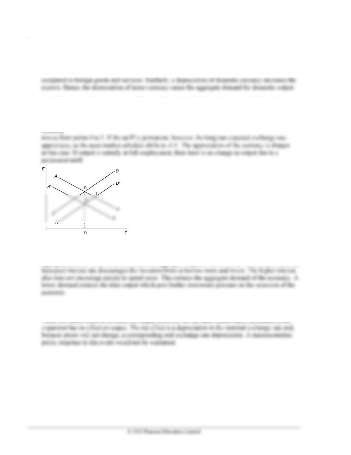
2. A tariff is a tax on the consumption of imports. The demand for domestic goods, and thus the level
of aggregate demand, will be higher for any level of the exchange rate. This is depicted in Figure 17(6)–
1 (below) as a rightward shift in the output market schedule from DD to DD. If the tariff is
temporary, this is the only effect, and output will rise even though the exchange rate appreciates as the
Figure 17(6)-1
3. Recession is a situation of low demand and output. Increased government expenditure increases the
aggregate demand which in turn increases the aggregate output of the economy. On the other hand, an
4. A permanent fall in private aggregate demand causes the DD curve to shift inward and to the left and,
because the expected future exchange rate depreciates, the AA curve shifts outward and to the right.
Chapter 17 (6) Output and the Exchange Rate in the Short Run 101
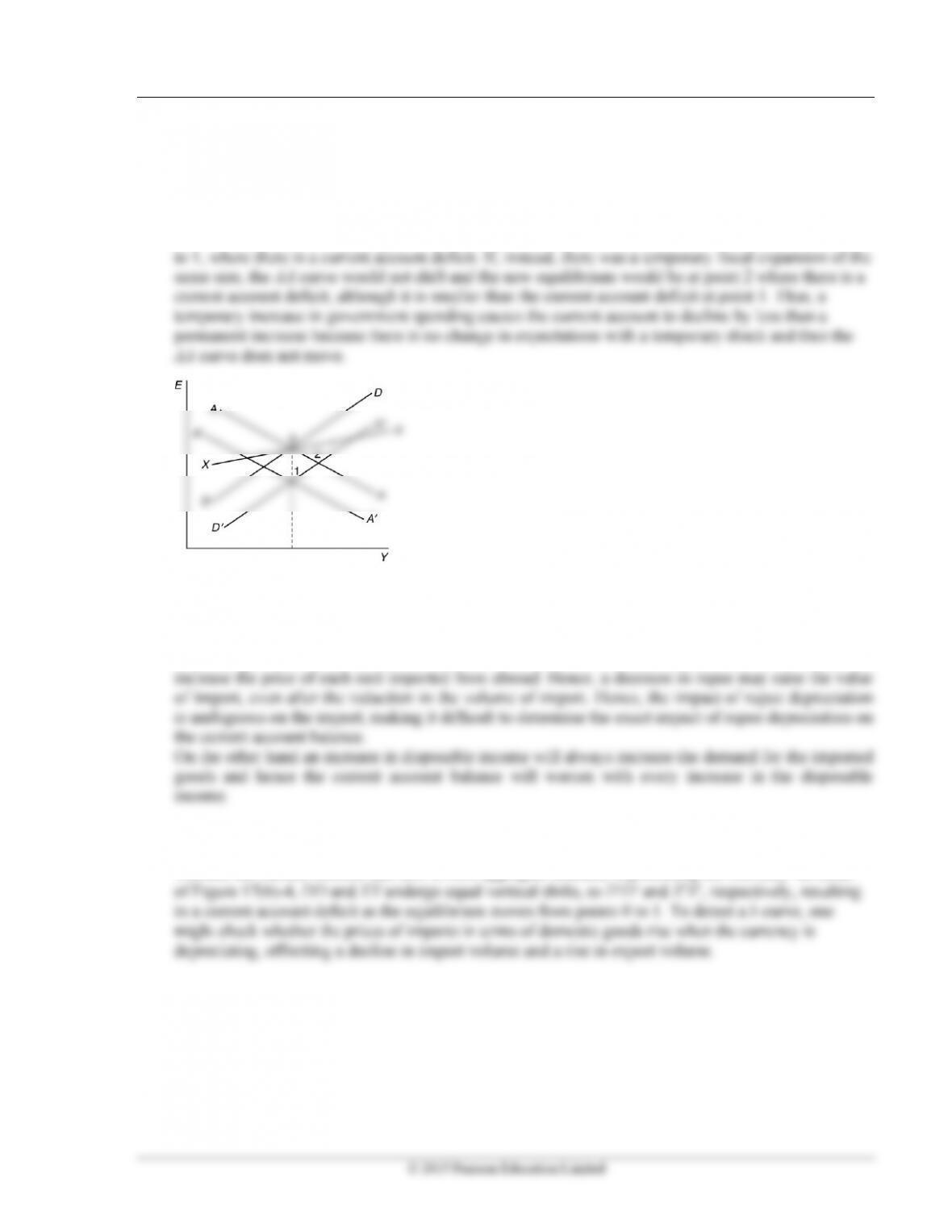
5. Figure 17(6)-2 (below) can be used to show that any permanent fiscal expansion worsens the current
account. In this diagram, the schedule XX represents combinations of the exchange rate and income
for which the current account is in balance. Points above and to the left of XX represent current
account surplus, and points below and to the right represent current account deficit. A permanent fiscal
expansion shifts the DD curve to DD and, because of the effect on the long-run exchange rate, the
AA curve shifts to AA. The equilibrium point moves from 0, where the current account is in balance,
Figure 17(6)-2
6. Current account balance is the difference between import and export. With rupee depreciation, Indian
products in the international market become less expensive. This increases India’s exports. At the
same time depreciation in the rupee makes the import expensive. This may reduce the demand for
imported goods, in terms of volume and not value. This is because, a depreciation of the rupee will
7. A currency depreciation accompanied by a deterioration in the current account balance could be
caused by factors other than a J-curve. For example, a fall in foreign demand for domestic products
worsens the current account and also lowers aggregate demand, depreciating the currency. In terms
102 Krugman/Obstfeld/Melitz • International Economics: Theory & Policy, Tenth Edition
© 2015 Pearson Education Limited
Figure 17(6)-4
8. The expansionary money supply announcement causes a depreciation in the expected long-run
exchange rate and shifts the AA curve to the right. This leads to an immediate increase in output
9. Increased inflation refers to a situation of high prices. An increase in price level reduces the real
money supply and drives the interest rate upward. Other things being equal, an increased interest rate
10. The derivation of the Marshall-Lerner condition uses the assumption of a balanced current account to
substitute EX for (q EX*). We cannot make this substitution when the current account is not initially
zero. Instead, we define the variable z = (q EX*)/EX. This variable is the ratio of imports to exports,
denominated in common units. When there is a current account surplus, z will be less than 1, and when
11. If imports constitute part of the CPI, then a fall in import prices due to an appreciation of the currency
will cause the overall price level to decline. The fall in the price level raises the real money supply.
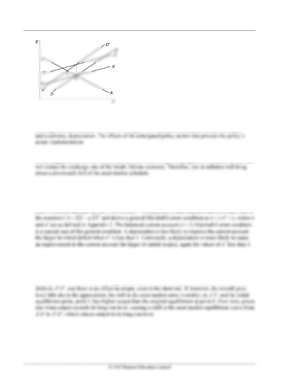
As shown in Figure 17(6)-6, the permanent fiscal expansion will shift the output market curve from
DD to DD and is matched by an inward shift of the asset market equilibrium curve. If import prices
are not in the CPI and the currency appreciation does not affect the price level, the asset market curve
Chapter 17 (6) Output and the Exchange Rate in the Short Run 103
© 2015 Pearson Education Limited
Figure 17(6)-6
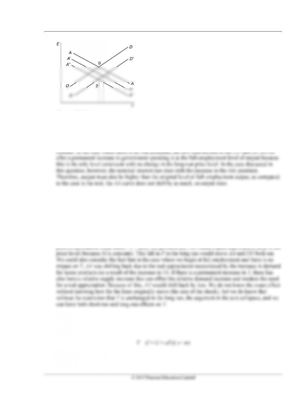
12. An increase in the risk premium shifts the asset market curve out and to the right, all else being equal.
A permanent increase in government spending shifts the asset market curve in and to the right
because it causes the expected future exchange rate to appreciate. A permanent rise in government
spending also causes the goods market curve to shift down and to the right because it raises aggregate
13. Suppose output is initially at full employment. A permanent change in fiscal policy will cause both
the AA and DD curves to shift such that there is no effect on output. Now consider the case where the
economy is not initially at full employment. A permanent change in fiscal policy shifts the AA curve
because of its effect on the long-run exchange rate and shifts the DD curve because of its effect on
expenditures. There is no reason, however, for output to remain constant in this case because its
initial value is not equal to its long-run level, and thus an argument like the one in the text that shows
the neutrality of permanent fiscal policy on output does not carry through. In fact, we might expect
that an economy that begins in a recession (below Yf) would be stimulated back toward Yf by a
14. We are given that the central bank in the economy can keep both interest rates and exchange rates
fixed. Thus, we need to only consider the goods side of the economy. The goods market equilibrium
is Y = (1 – s)Y + I + G + aE – mY. Collecting terms and solving for Y yields:
104 Krugman/Obstfeld/Melitz • International Economics: Theory & Policy, Tenth Edition
© 2015 Pearson Education Limited
Thus, a 1 unit increase in government spending will cause output to increase by 1/(s + m). Recall that
s is the marginal propensity to save and m is the marginal propensity to import. As both of these
marginal propensities increase, the multiplier effect of government spending will decrease. This
makes intuitive sense as the impact of government spending will be diluted if some of that spending
is saved (s) and if some of that spending leaves the country through imports (m).
15. The text shows output cannot rise following a permanent fiscal expansion if output is initially at its
long-run level. Using a similar argument, we can show that output cannot fall from its initial long-run
level following a permanent fiscal expansion. A permanent fiscal expansion cannot have an effect on
the long-run price level because there is no effect on the money supply or the long-run values of the
domestic interest rate and output. When output is initially at its long-run level, R equals R*, Y equals
Yf, and real balances are unchanged in the short run. If output did fall, there would be excess money
6. Liquidity trap is a situation where the short term interest rate is close to zero. When the central bank
goes for the expansionary monetary policy by increasing the money supply, it reduces the interest rate
to zero. At zero interest rate, people are indifferent between the money and bonds. The lowered
interest rates reduce the lure of bonds; people prefer to hold more disposable money instead of buying
bonds. When the interest rate is zero, any further purchases of bonds by the central bank won’t affect
the output level in the economy. The interest rate will not go below zero because the currency itself
17. High inflation economies should have higher pass-through as price setters are used to making adjustments
faster (menu costs fall over time as people learn how to change prices faster). Thus, a depreciation in
a high-inflation economy may see a rapid response of changing prices, but firms in a low-inflation
18. An increase in fiscal expenditure increases the income level in the economy; therefore, it shifts the
demand schedule to right without affecting the Asset market schedule. This increases the level of
output and appreciates the domestic currency (figure 17.11). When there is a change in the taste of
domestic consumers towards foreign products, the demand for the domestic product declines causing
19. Many answers are possible.
20. Many answers are possible.