17 Balance of Payments I: The Gains from Financial Globalization
Notes to Instructor
Chapter Summary
This chapter connects the balance of payments to long-run economic growth and
highlights the benefits of international finance for consumption smoothing, investment,
and risk sharing. The key lessons from this chapter are as follows:
■ An open economy is able to smooth consumption through borrowing or lending,
affecting its current account and external wealth position.
■ Even when countries are unable to borrow or lend internationally, they can share
risk through diversifying their portfolio of capital across countries.
Comments
This chapter makes heavy use of present value and intertemporal trade–offs. Students
may find this material unfamiliar. Instructors will find it useful to review the basic
concept of present value and to highlight the difference between thinking in a dynamic
model and thinking in a static one. Also, students may be intimidated by the math used in
this chapter because it is somewhat technical.
The section is broadly organized as follows:
1. The Limits on How Much a Country Can Borrow: The Long-Run Budget
Constraint
a. How the Long-Run Budget Constraint Is Determined
vi. Extending the Theory to the Long Run
b. A Long-Run Example: The Perpetual Loan
c. Implications of the LRBC for Gross National Expenditure and Gross
Domestic Product
d. Summary
e. Application: The Favorable Situation of the United States
iv. Too Good to Be True?
2. Gains from Consumption Smoothing
a. The Basic Model
b. Consumption Smoothing: A Numerical Example and Generalization
i. Closed Versus Open Economy: No Shocks
c. Summary: Save for a Rainy Day
d. Side Bar: Wars and the Current Account
3. Gains from Efficient Investment
a. The Basic Model
b. Efficient Investment: A Numerical Example and Generalization
i. Generalizing
c. Summary: Make Hay While the Sun Shines
d. Application: Delinking Saving from Investment
Countries?
iv. An Augmented Model: Countries Have Different Productivity Levels
f. Application: A Versus k
i. More Bad News?
g. Side Bar: What Does the World Bank Do?
4. Gains from Diversification of Risk
a. Diversification: A Numerical Example and Generalization
i. Home Portfolios
b. Application: The Home Bias Puzzle
c. Summary: Don’t Put All Your Eggs in One Basket
6. Appendix: Common Versus Idiosyncratic Shocks
An alternative organization for class lecture is given in the following. This combines
1. The Limits on How Much a Country Can Borrow: The Long-Run Budget
Constraint
2. Gains from Consumption Smoothing
3. Gains from Efficient Investment
4. Linking the LRBC to Economic Growth and Investment
a. Can Poor Countries Gain from Financial Globalization?
5. Linking the Model to Risk Diversification
6. Appendix: Common Versus Idiosyncratic Shocks
Lecture Notes
Now that we have covered the accounting of international transactions, we are prepared
to analyze their meanings in two different contexts: the long run (this chapter) and the
short run (the following chapter).
When a country seeks to increase investment, this involves a difficult trade–off.
Although investment is key to economic growth and prosperity, investing in capital
resources today requires giving up consumption. In the same way that an individual takes
S = I + CA
This chapter shows how open economies can benefit from financial globalization
through borrowing or saving with other countries to (1) smooth consumption and (2)
1 The Limits on How Much a Country Can Borrow: The Long–Run Budget
Constraint
We know from the previous chapter that borrowing or lending internationally has
implications for external wealth. This chapter extends the analysis of external wealth to
study how this variable evolves over time, using the intertemporal approach.
Understanding how countries lend and borrow is easy once household lending and
loan amount is reduced with each payment, over the life of the loan, the fraction of each
payment that is principal rises, while the fraction that is interest falls. The final payment
is mostly principal with just a bit of interest. Consider two cases:
■ Case 1 A debt that is serviced. The household makes interest payments on the
Case 2 is not sustainable because it assumes one can borrow a larger and larger amount
each year by rolling over the amount owed each period. This is also known as a pyramid
How the Long–Run Budget Constraint Is Determined
We begin with the assumptions used in the model:
■ Prices are perfectly flexible. This means the model can be defined in real terms,
■ The country is a small open economy. This means the country’s behavior
(borrowing or lending) does not affect prices or interest rates in world markets
and that there are no capital controls.
■ All debts carry a real interest rate r*, the world real interest rate.
Calculating the Change in Wealth Each Period Consider the change in external wealth
in a given period, N:
This expression says that external wealth will change from two sources: trade deficits or
surpluses and net interest income earned on external wealth from the previous period.
Calculating Future Wealth Levels Adding WN−1 to both sides yields the following
expression for external wealth in period N:
This expression can be applied to calculate future external wealth based on the country’s
trade balance, TBN, and initial external wealth, WN−1.
The Budget Constraint in a Two–Period Example Suppose there are two periods in the
economy. The current period denoted is 0 (= N) and the previous period is denoted −1 (=
The next period is denoted 1 (= N + 1):
Substituting in the expression for current external wealth, W0, we get
Note that the country’s external wealth in period 1 depends on the amount of external
wealth accumulated through net interest income earned and the trade balance each period
prior. Now, if we assume that all debts must be repaid, then the country should have no
external wealth in the last period (period 1 in this case), W1 = 0. Based on this
assumption, we have the following:
Present Value Form The previous expression can be rewritten by dividing both sides by
(1 + r*):
A Two–Period Example The previous expression shows that the present value of future
trade balances must be equal to the negative of the present value of wealth from the last
period, −(1 + r*)W−1. In other words:
then this country is a net lender and therefore can afford to run future trade
deficits because it initially has positive external wealth.
then this country is a net debtor and therefore must run trade surpluses to pay off
its debts.
Extending the Theory to the Long Run It’s straightforward to extend the two-period
case to N periods. The LRBC becomes
If students feel comfortable with summation notation, it can be expressed as
This expression says that an initial credit or debit must be balanced by offsetting trade
surpluses or deficits in the future. Again, it is worth highlighting that the stream or sum of
A Long–Run Example: The Perpetual Loan
This example considers a perpetual loan in which a country pays a fixed amount, X, each
period, beginning in period 1 and lasting forever. This is a useful case to study because it
is equivalent to Case 1 from the beginning of the chapter (e.g., the principal is rolled
over, while the borrower pays interest that accrues each year). The present value of this
stream of payments is expressed as
Multiply both sides by (1 + r*):
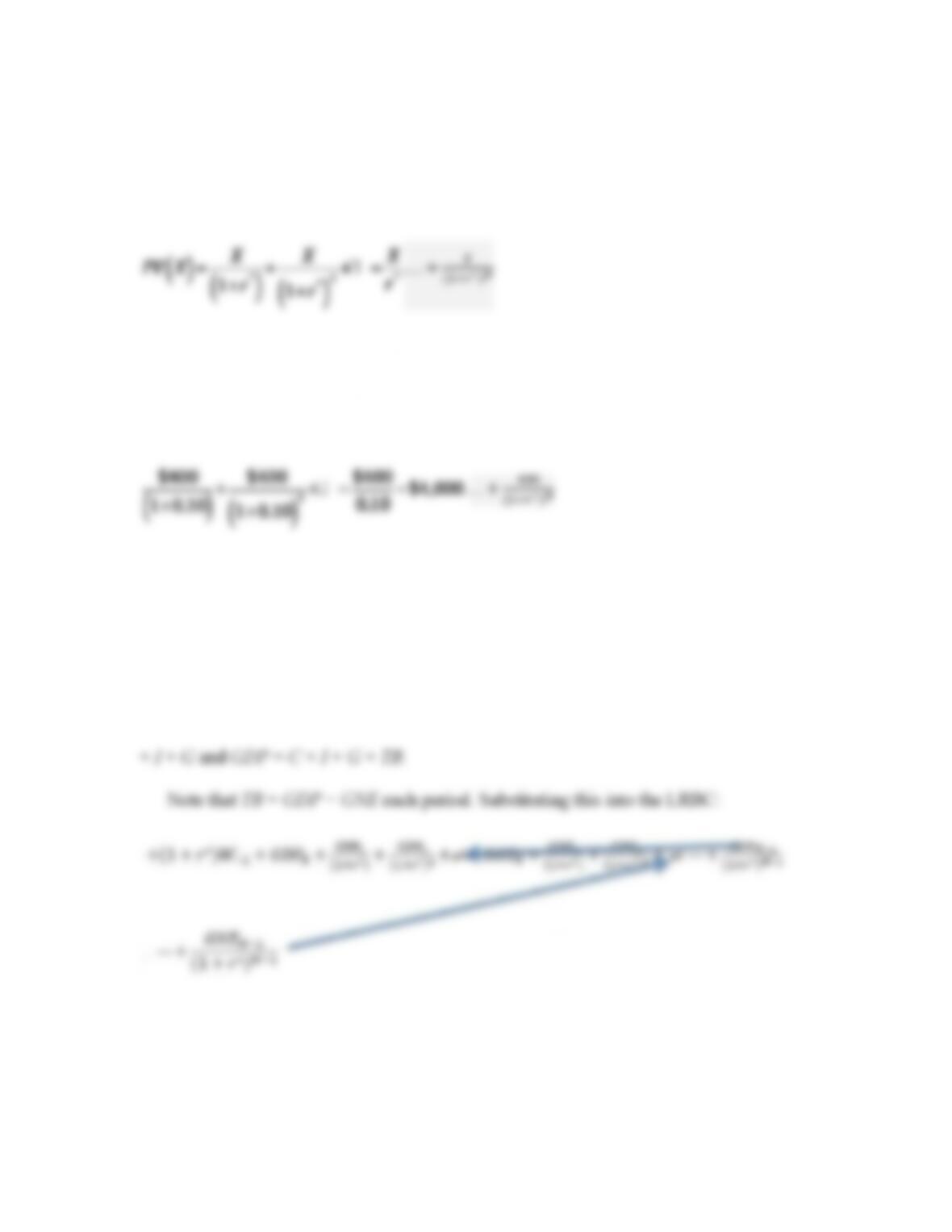
Subtracting the first expression from the second one, we see PV(X) = X/r*:
For example, consider a fixed payment of $400 at an interest rate of 10%:
Implications of the LRBC for Gross National Expenditure and Gross Domestic
Product
Now that we are familiar with how external wealth changes over time and how this
relates to trade balances, we can use the LRBC to understand the link between GNE = C
The LRBC says that in the long run, in present value terms, a country’s expenditures
(GNE) must equal its production (GDP), plus any initial wealth.
This shows how a country is able to finance the differences between its production
Summary
In a closed economy, TB = 0, so production and expenditure must be equal. In an open
economy, a country can spend more than it produces by borrowing, or it can produce
APPLICATION
The Favorable Situation of the United States
Recall two key assumptions from the LRBC: the same, constant real interest rate, r*,
“Exorbitant Privilege” Since the 1980s, the United States has been a net debtor, r*W <
0, yet net factor income from abroad has been positive during this period. How does a net
debtor earn positive interest income?
The U.S. earns interest at the world interest rate r* on its external assets but pays
“Manna from Heaven” In addition to the difference in interest rates on assets and
liabilities, the United States has consistently enjoyed capital gains on external wealth.
This amounts to roughly 2 percentage points in net capital gains (net of capital losses on
Summary The United States has earned about 3.5% per year more than the rest of the
world (earning 2% in capital gains plus 1.5% more in interest). This has been going on
since the 1980s. The total return differential was near zero for every other G7 country.
We can modify the LRBC to relax the two assumptions about interest rates and
capital gains:
Too Good to Be True? The two additional effects in the previous expression show how
diminishing over time.
Research by Daniel Gros seems to show that the United States borrowed $5.5 trillion
between 1986 and 2006. However, U.S. external wealth as reported had fallen by only
APPLICATION
The Difficult Situation of the Emerging Markets
In the previous application, we saw that applying the LRBC model to the United States
required relaxing some assumptions. If we consider emerging markets, we similarly must
relax the model’s assumptions to account for special situations in these countries. This
application considers two assumptions: (1) the interest rates paid on assets and liabilities,
risk premium (e.g., compare Italy to Israel and Jamaica).
■ As public debt rises, the bond ratings fall much more for non-advanced countries
(e.g., compare Austria and the United States to Poland and India).
2 Gains from Consumption Smoothing
This section uses the LRBC together with a simple model of an economy to illustrate
The Basic Model
This section uses the same assumptions as outlined at the beginning of the LRBC section.
In addition:
■ GDP = Q produced using a single input: labor.
■ Analysis begins in period 0, with given initial wealth equal to zero, W−1 = 0.
■ The country is small, the rest of the world (ROW) is large, and the prevailing
world interest rate is constant at r* = 5%.
Based on these assumptions:
Consumption Smoothing: A Numerical Example and Generalization
We consider two cases to see how a country can smooth consumption:
The following examples use the same numerical values as those used in the textbook. For
a complete discussion of common versus idiosyncratic shocks, see the appendix. The
following discussion examines idiosyncratic shocks.
Closed Versus Open Economy: No Shocks
■ Closed economy: Q = 100 = C
In an open economy with no shocks, there is no reason to borrow or lend. The country is
able to maintain smooth consumption every period.
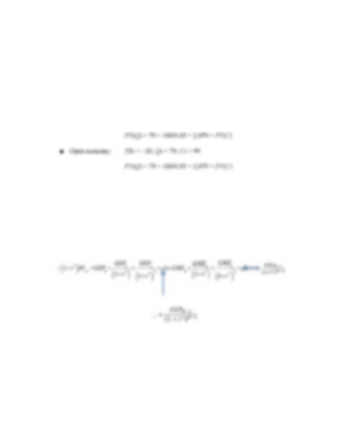
Closed Versus Open Economy: Shocks Suppose there is a temporary negative shock to
output, or −21 units. Output is equal to 100 units in every period afterward.
■ Closed economy: Q0 = 79 = C0
Note that in the open economy, the present value of output is the same, yet the country is
able to smooth consumption by running a trade deficit in the period when the negative
shock reduces output.
How to solve for the numerical values. We can use the LRBC equation:
Based on our assumptions, this expression simplifies to
Or, using the formula for a perpetual loan, we get
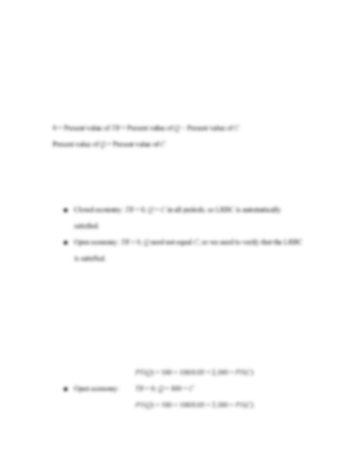
Because the country begins with initial external wealth equal to zero, the present value of
the trade balance must be equal to 0, that is, the present value of consumption must be
equal to the present value of output:
PV(Q) = PV(C)
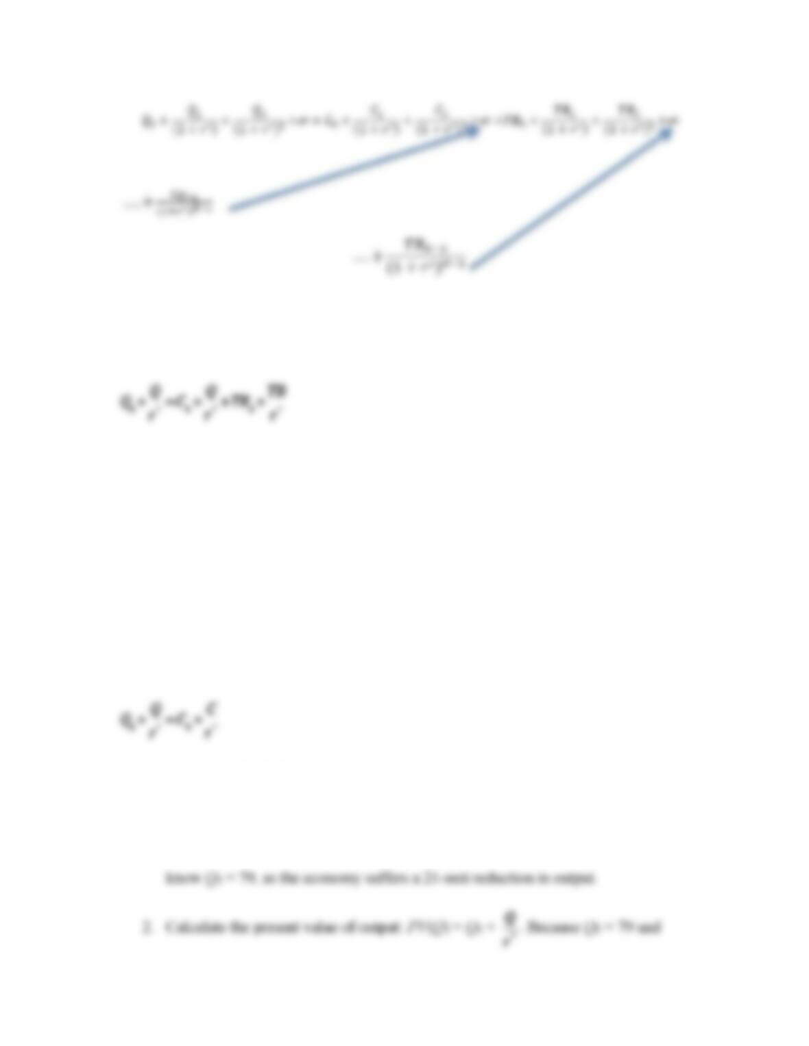
Steps to computing numerical values for Q, C, TB, NFIA, and W over time are as follows:
1. Identify the initial level of output (as a result of the shock). From the example, we