hold.
Changes in the nominal exchange rate reflect:
■ Inflation differentials
2 Exchange Rates in the Short Run: Deviations from Uncovered Interest
Parity
The UIP condition relies on arbitrage to ensure that the expected return on foreign
deposits equals the return on domestic deposits in the same currency terms. There is still
APPLICATION
The Carry Trade
UIP: Home interest rates should equal the foreign interest rate plus the expected rate of
depreciation in the home currency. If UIP holds, an investor cannot earn riskless profit
from borrowing in one currency and investing in another. This type of investment
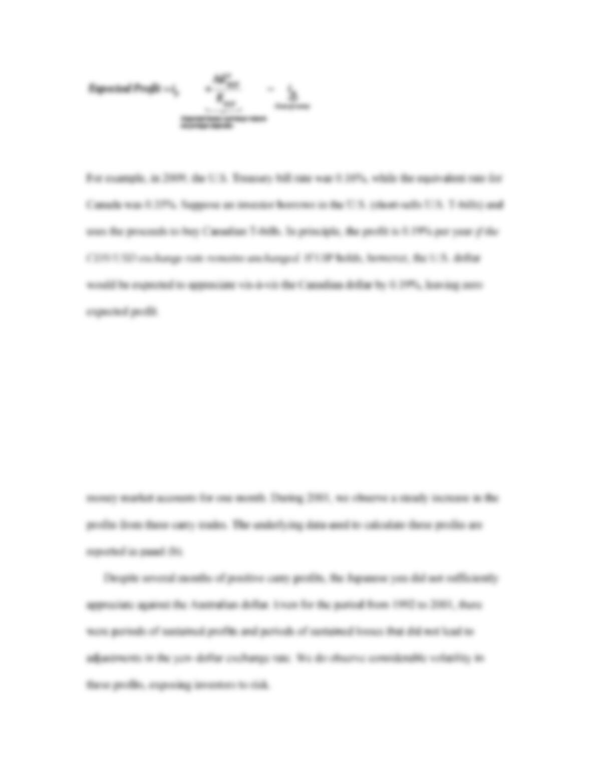
strategy is called carry trade, with expected profits defined as the difference in returns:
The Long and Short of It In practice, investors do engage in carry trade and earn large
profits from doing so. Investors borrow in low-interest currencies (“go short”) and invest
in higher-interest currencies (“go long”).
Figure 22-4, panel (a), reports profits from carry trade involving borrowing in the
low-interest Japanese yen money market and investing in high-interest Australian dollar
Using some language from financial markets, we can consider the role of leverage
and margin. Suppose that you have $2,000 to invest and borrow an additional $48,000 in
Carry Trade Summary We observe the following from carry trade data:
■ Even if expected returns from arbitrage are equal to zero, actual profits are often
not equal to zero.
H E A D L I N E S
Mrs. Watanabe’s Hedge Fund
This article summarizes the 2006–2007 experiences of individual Japanese investors with
carry trade.
Background:
Total profits from carry trade involving the yen totaled $4 trillion in 2006, according to
an OECD estimate.
■ Middle-class Japanese homemakers, “Mrs. Watanabes,” have engaged in currency
Key statistics:
■ Japanese homemakers are largely responsible for managing the nation’s $12.5
trillion in household savings.
■ A small fraction of these savings is invested in currency speculation, margin
Lessons:
■ Carry trade involves considerable risk.
Discussion questions:
■ Consider the data reported in Figure 22-4. Do you expect that margin trading
involving borrowing in yen and investing in Australian dollars will be profitable
in the long term? Why might currency traders engage in these activities in the
immediate term?
■ Is the experience reported in the article consistent with UIP?
APPLICATION
Peso Problems
It’s possible to earn positive returns trading currencies that are pegged. For example, both
Hong Kong’s dollar and many countries in the Middle East and the Caribbean are pegged
Hong Kong:
■ Panel (a) shows the interest rate differential between Hong Kong and the U.S. was
near zero most of the time. Hong Kong’s peg was considered the most solid in the
world.
bank was able to defend the peg. The expected depreciation never happened.
■ Investors who believed the Hong Kong dollar would maintain its value could
Argentina:
■ In 2001, an economic and banking crisis led to worries of default, driving down
the value of the Argentine peso.
■ The IMF pressured Argentina’s government to use monetary policy for purposes
other than defending the exchange rate peg, further driving up the currency +
The peso problem refers to the currency premiums associated with a pegged currency.
The collapse of a peg can be viewed as infrequent, and even unlikely, as in the case of
The Efficient Markets Hypothesis
This section develops a familiar model from financial economics: the efficient markets
hypothesis. The model is used to examine whether carry trade profits disprove UIP.
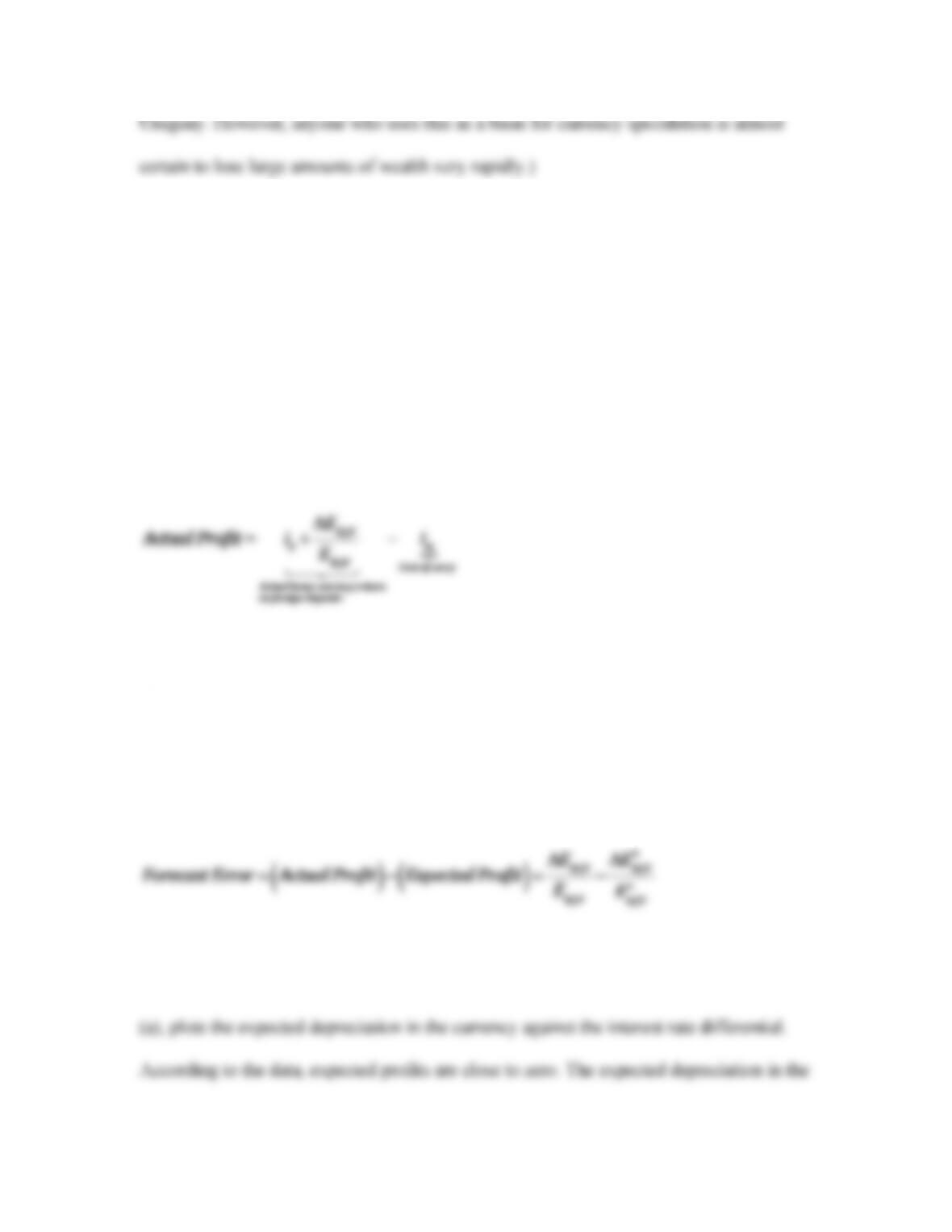
We observed from the data that arbitrage means expected ex ante profits should be
equal to zero. The actual ex post profit is expressed as
The actual exchange rate is used to determine the profit or loss earned by the investor
engaged in carry trade. The difference between the actual and expected profit is the
forecast error:
Expected Profits The UIP condition has to do with ex ante profits. Figure 22-6, panel
Actual Profits Figure 22-6, panel (b), reports the actual depreciation against the interest
rate differential. From this figure, we see that actual profits are made and that the data are
The UIP Puzzle By itself, the fact that profits are positive does not imply UIP is
incorrect. If the distribution of profits is random, UIP would hold on an expected value
A related theory, the efficient markets hypothesis, says that financial markets are
An empirical test of UIP combined with the rational expectations and efficient
markets hypothesis fails, suggesting the forex market is an inefficient market. This
leaves us with the question, if there are forecastable profits available in the forex market,
why don’t investors arbitrage away these profits?
Note to instructor: A more in–depth presentation of the efficient markets and rational
Limits to Arbitrage
The explanations for the existence of predictable profits are based on limits to arbitrage.
Trade Costs Are Small It’s tempting to simply list the same frictions we saw earlier in
this chapter: trade costs, nontraded goods, and the speed of convergence to equilibrium.
A related issue has to do with the liquidity of the foreign currency. An attempt to
trade a large quantity of a less liquid currency may cause the exchange rate to change.
Thus, for example, buyers who want to acquire $1 million of Albanian leke should expect
Risk Versus Reward We can look at the relationship between the profits earned on carry
trade and compare these returns with the risks to which investors are exposed. Using the
data reported in Figure 22-6, panel (b), we observe that a positive 1% interest differential
The Sharpe Ratio and Puzzles in Finance Carry trade profits are the difference
between risky foreign rates of return and safer domestic returns. An excess return is
earned on that difference. We can use one of the standard tools of finance to help us
A higher ratio indicates that an asset with a given level of risk earns a higher return. A
lower ratio suggests the asset has a low return relative to the degree of risk.
Figure 22-7 reports carry trade returns, volatility, and Sharpe ratios for selected
currencies relative to the British pound, as well as for a market portfolio of all these
currencies. We observe the following:
■ Returns are positive for all these currencies; equal to roughly 4% per year.
■ The standard deviation of these returns is very high, with an average of 6%.
Research in behavioral finance on why investors do not arbitrage away these profits
focuses on rectifying seemingly irrational market outcomes.
Predictability and Nonlinearity We have already seen that trade costs are too small and
that the risk‒reward trade-off cannot explain the existence of predictable profits in the
forex market. Perhaps the linear model is a poor description of the forex market.
Conclusion
The data show there are predictable, positive returns in the forex market. By itself, this is
not a violation of UIP. When we add efficient markets, the existence of such profits
3 Debt and Default
This section examines the role of sovereign default in international capital markets.
Sovereign default occurs when a sovereign government fails to meet its obligations to
make payments on debt held by foreigners.
Sovereign defaults have a very long history:
■ Greek municipalities defaulted on loans from the Delos Temple in the fourth
century BC.
■ In 1343, England defaulted on a debt owed to Florence merchants. As a result, the
■ The U.S. federal government has avoided default during its short history, although
individual states have defaulted when they were emerging markets during the
19th century.
Today’s advanced economies do not default, but it is a recurring problem in emerging
markets and developing countries:
■ Argentina, Brazil, Mexico, Turkey, and Venezuela have defaulted five to nine
Puzzle: Why do emerging markets and developing countries get into default trouble at
lower levels of debt relative to advanced economies?
■ As of late 2010, a number of European countries have gone to the brink of
A Few Peculiar Facts About Sovereign Debt
Debtors are almost never forced to pay. There is virtually no way to force a sovereign
government to honor its debt obligations. Repayment of debt is largely a choice for the
borrowing government. How painful does repayment have to get before default occurs?
We need to evaluate the costs and benefits associated with default versus repayment.
The benefit is, obviously, that the country keeps the funds borrowed and does not have to
repay anything. What are the costs?
■ Financial market penalties:
● Debtors that default are excluded from credit markets for some period after
■ Broader macroeconomic costs:
● Lost investment, lost trade, or lost output caused by adverse financial market
Summary Sovereign debt is a contingent claim: governments will repay only if the
A Model of Default, Part One: The Probability of Default
Assumptions In the model, a country will borrow to smooth its consumption. Repayment
of the debt is contingent on losses associated with output fluctuations.
■ Fluctuations in output are exogenous, with output, Y, taking on some value
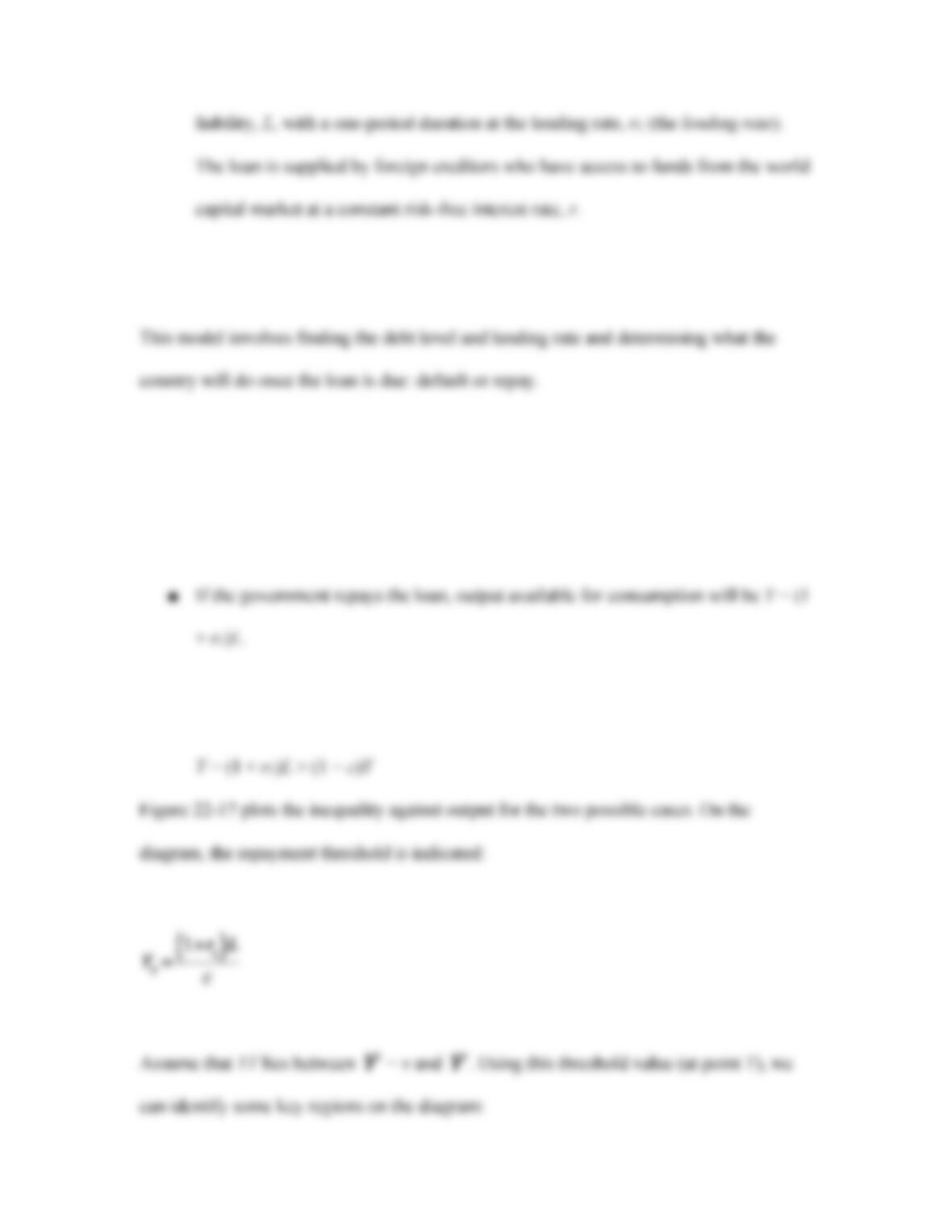
■ The loan balance is due at the end of period 1, the period in which output
declines.
The Borrower Chooses Default Versus Repayment Assume the borrower suffers some
cost associated with defaulting, cY, leaving (1 − c)Y available for consumption. The
choice facing the government is whether to default or repay the loan.
■ If the government defaults, it has (1 − c)Y available for consumption. Therefore,
the condition for repayment is
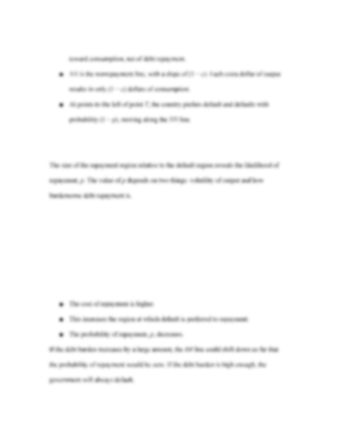
■ RR is the repayment line, with a slope of 1. Each extra dollar in output goes
■ At points to the right of point T, the country prefers repayment and repays with
probability p, moving along the RR line.
An Increase in the Debt Burden Suppose there is an exogenous increase in the debt
burden. (This could be caused by an increase in the lending rate, an increase in the
volume of borrowing, or some combination of the two.) The new burden is (1 + r
′
L)L
′
.
This scenario is shown in Figure 22-9.
■ The RR line shifts down to R
′
R
′
.
An Increase in Volatility of Output Suppose the potential decrease in output is larger,
so V increases to V
′
. This case is illustrated in Figure 22-10.
■ Consumption levels along RR and NN are unaffected.
The Lender Chooses the Lending Rate Based on the probability of repayment, we can
determine the interest rate the lender will charge for a loan. Competition in financial
markets means that lenders simply will break even, so the lender will set the interest rate
such that the revenues exactly equal the costs. The break-even condition follows:
■ If p = 100%, the loan is risk-free, and rL = r.
APPLICATION
Is There Profit in Lending to Developing Countries?
22-20 reports the results of this analysis of ex post returns.
■ Average returns = 9.1% per year:
■ Based on typical risk premium estimates from 1998 to 2007, an extra 2.8% return
A Model of Default, Part Two: Loan Supply and Demand
This model will be useful in analyzing the equilibrium behavior of loans, the interest rate
charged on these loans, and the probability of repayment.
Loan Supply Suppose that output volatility, V, is low. The probability of repayment is

■ When the loan amount is low, less than some value LV:
● the loan will be repaid with 100% probability.
■ As the loan amount increases, above LV (but below LMAX):
● the probability of loan repayment decreases.
■ When the loan amount is high, above some value LMAX:
Loan Demand The slope of LD(V) depends on two factors: the lending rate, rL, and
output volatility, V. Figure 22-21, panel (b), illustrates loan demand as a decreasing
function of the lending rate, rL.
The equilibrium in the loan market is shown as Point 3 in Figure 22-21, panel (b). We
An Increase in Volatility Figure 22-22 illustrates how an increase in output volatility
affects loan demand.
■ Panel (a):
● An increase in V leads to an increase in the probability of default. As V rises,
the probability of repayment drops below 100% at a lower level of debt.
● The probability of repayment function shifts left.
■ Panel (b):
● Loan supply decreases: For a given loan amount, L (above L
′
V and below
LMAX), the equilibrium lending rate is higher because: