Spherical Potential Equation Example (10)
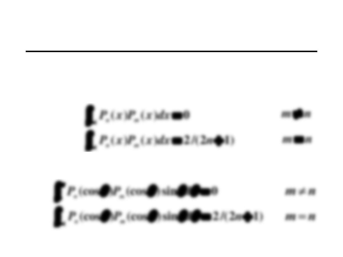
We can find coefficients satisfying Equation 10 because
Legendre polynomials form yet another orthogonal set
Equivalently
n
c
Spherical Potential Equation Example (11)
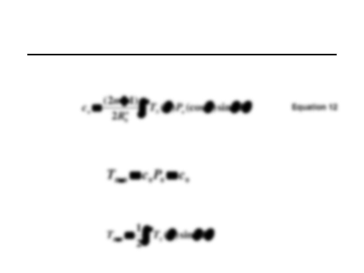
The coefficient satisfying Equation 11 is given by
From Equation 10 we see that the temperature at the center of this
“world” is
and from Equation 12 we see that this is
n
c
Spherical Potential Equation Example (12)
Take-aways (What’s important here?):
You should know:
How to separate variables as a method of solving PDEs

Partial Differential Equations
Beam Equation
Beam Equation
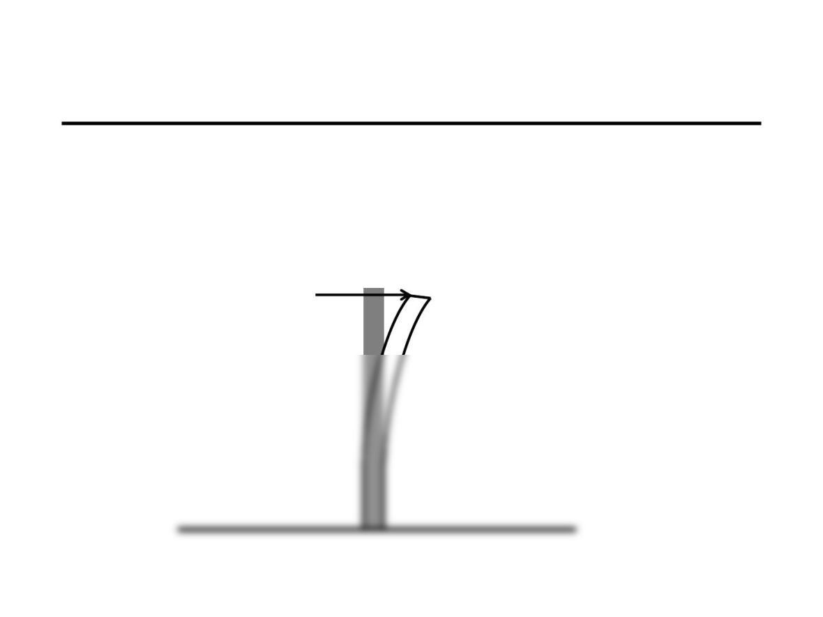
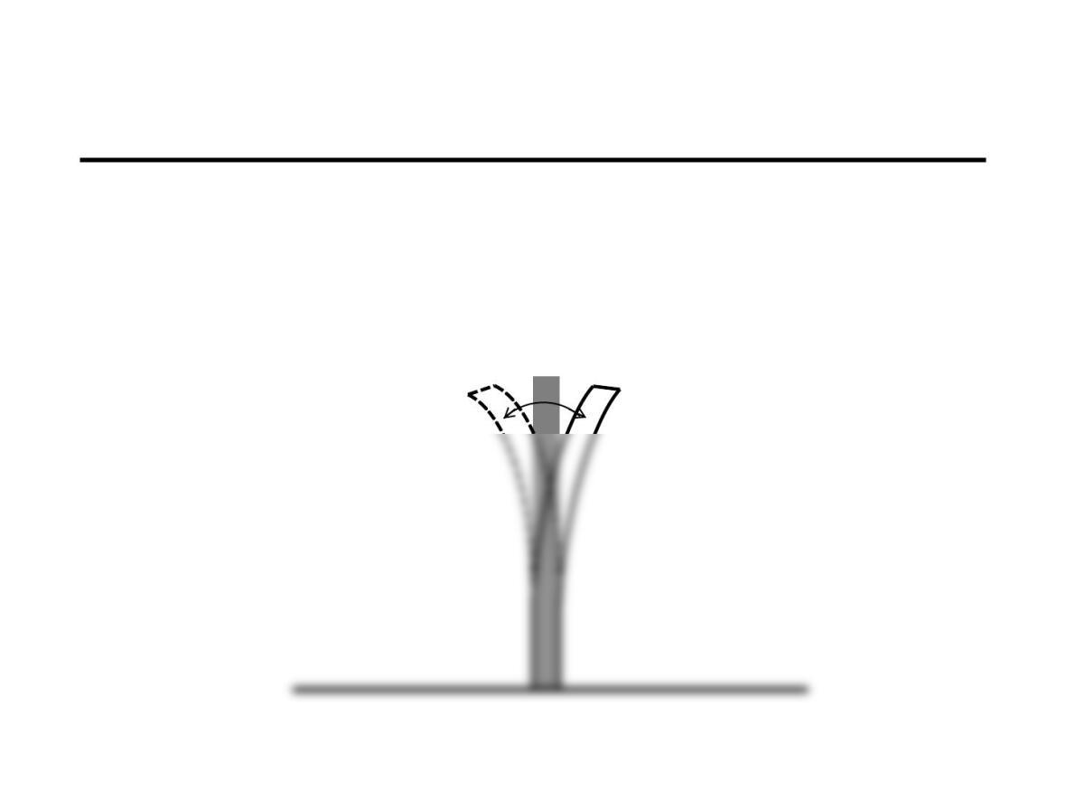
Consider a cantilever beam of length and uniform cross-section
initially depressed with a point load at the end and then released
to vibrate freely.
h
Beam Equation (2)
This model is somewhat similar to an aircraft wing in turbulence and
a skyscraper after the shock of an earthquake.
Beam Equation (3)
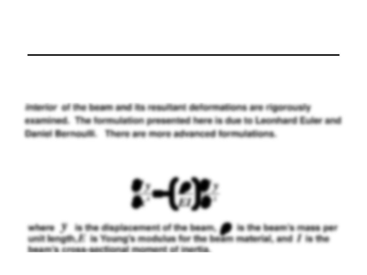
Scientific analysis of bending motions in a continuous beam is found
in solid mechanics. In that discipline, the forces and moments in the
The Euler-Bernoulli beam equation is
beam’s cross-sectional moment of inertia.
Beam Equation (4)
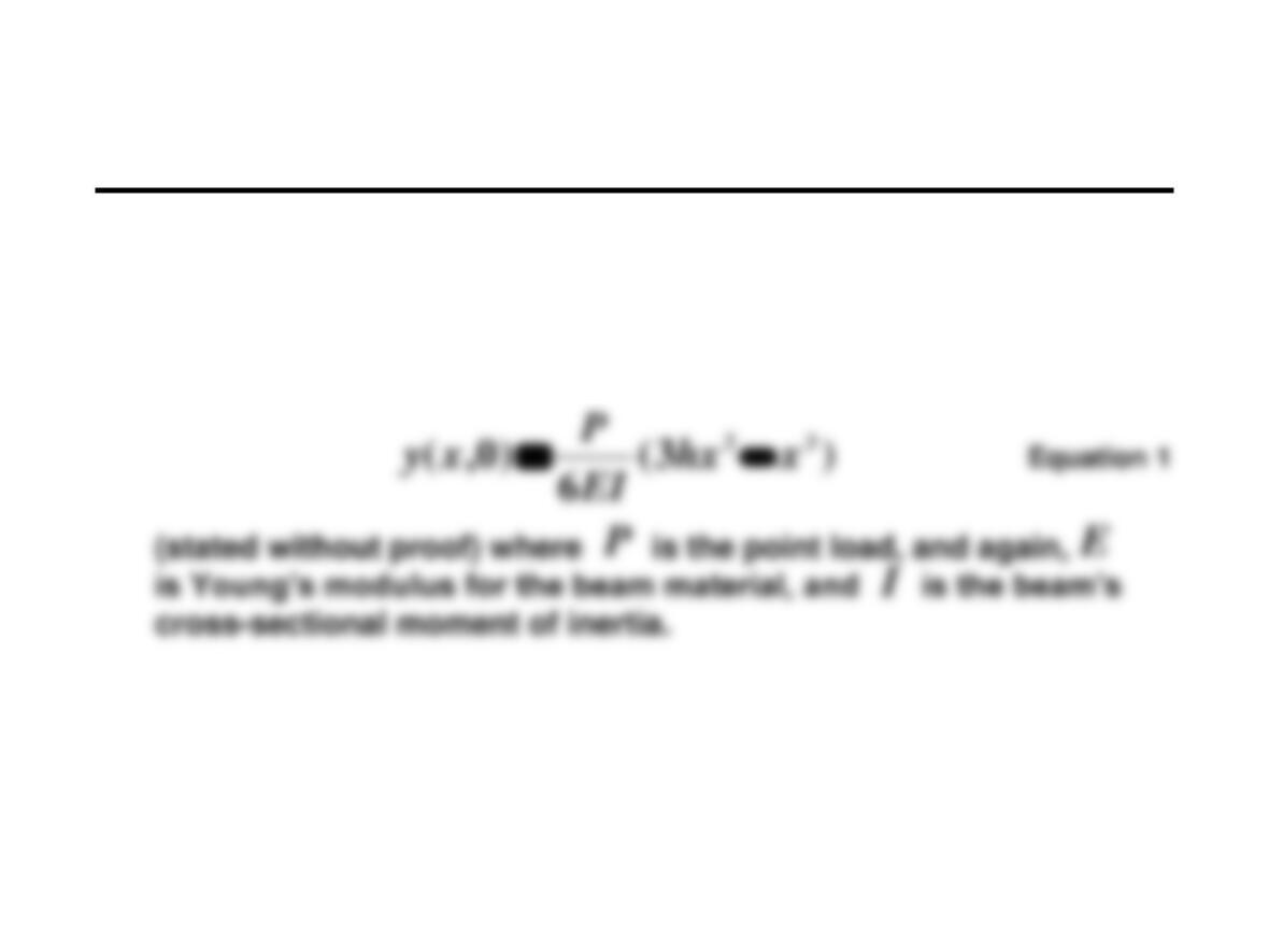
The displacement from vertical along the beam is initially given by
Analysis of Beam Motion
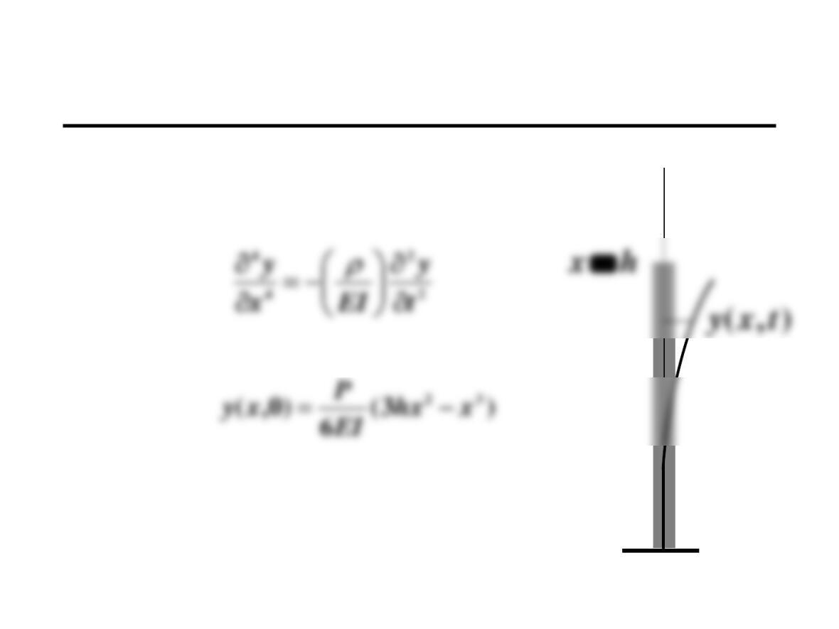
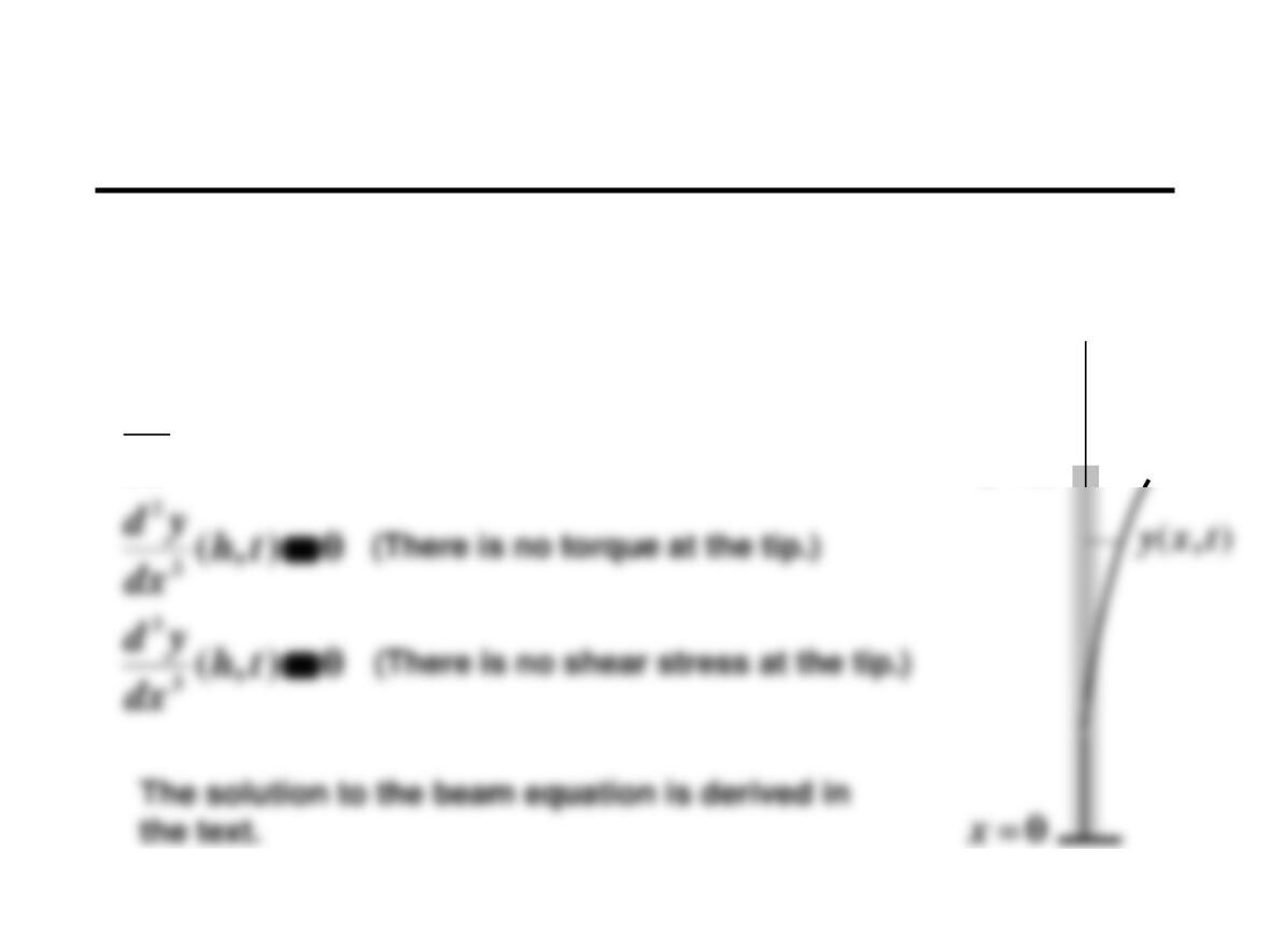
The equations to be solved are
with initial condition
and boundary conditions (which require
knowledge of solid mechanics) as given
on the next chart
x
0=x
Analysis of Beam Motion (2)
x
hx =
0),0(
0),0(
=
=
t
dx
dy
ty
(The base is held stationary.)
(The beam remains vertical at its base.)
Analysis of Beam Motion (3)
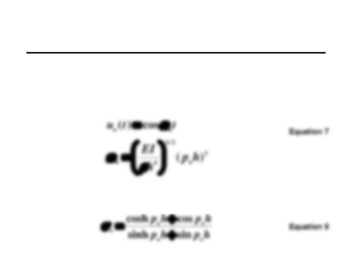
In summary, the solution is
where
=
=
1
)()(),(
n
nnn tuxwctxy
)sin(sinhcoscosh)( xpxpxpxpxw nnnnnn −−−=
Equation 6
Equation 8
Analysis of Beam Motion (4)
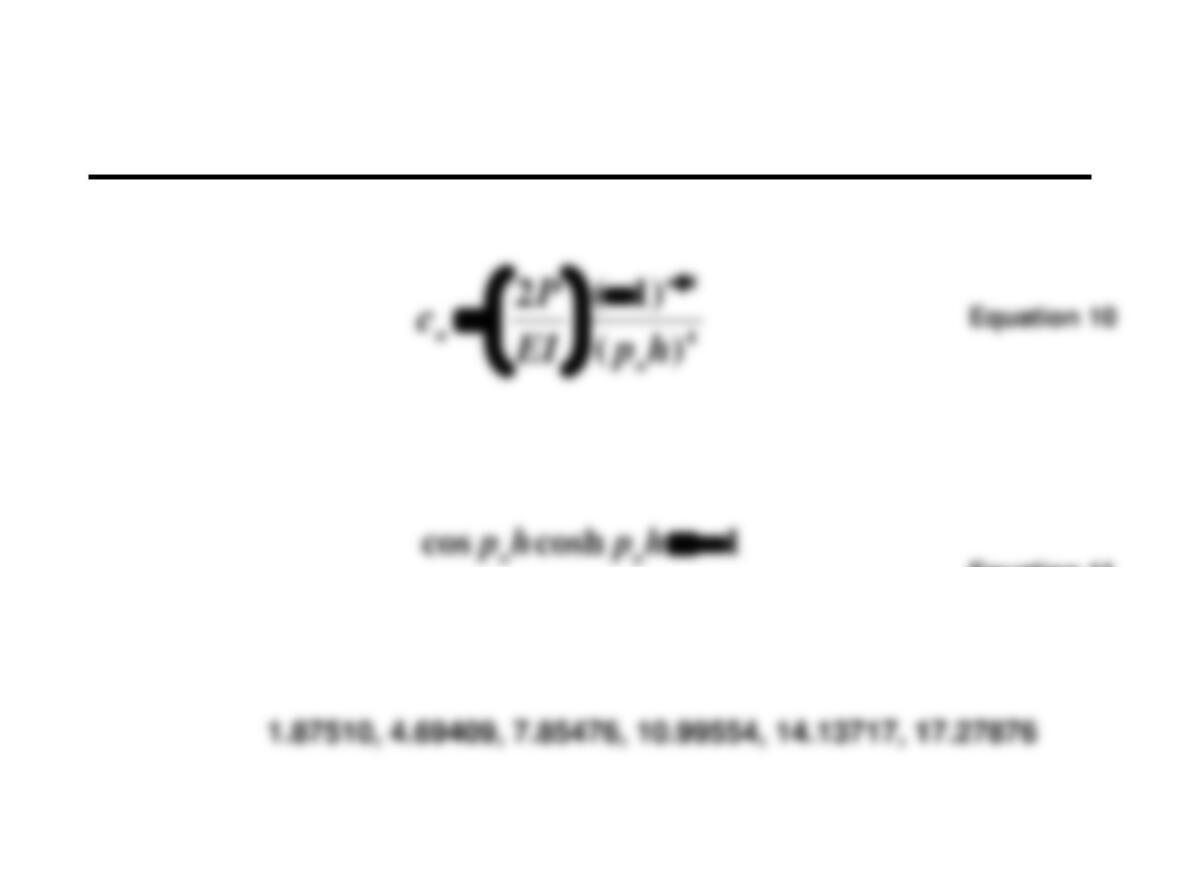
and is the nth solution to
the first six of which are
hpn
Equation 11
Analysis of Beam Motion (5)
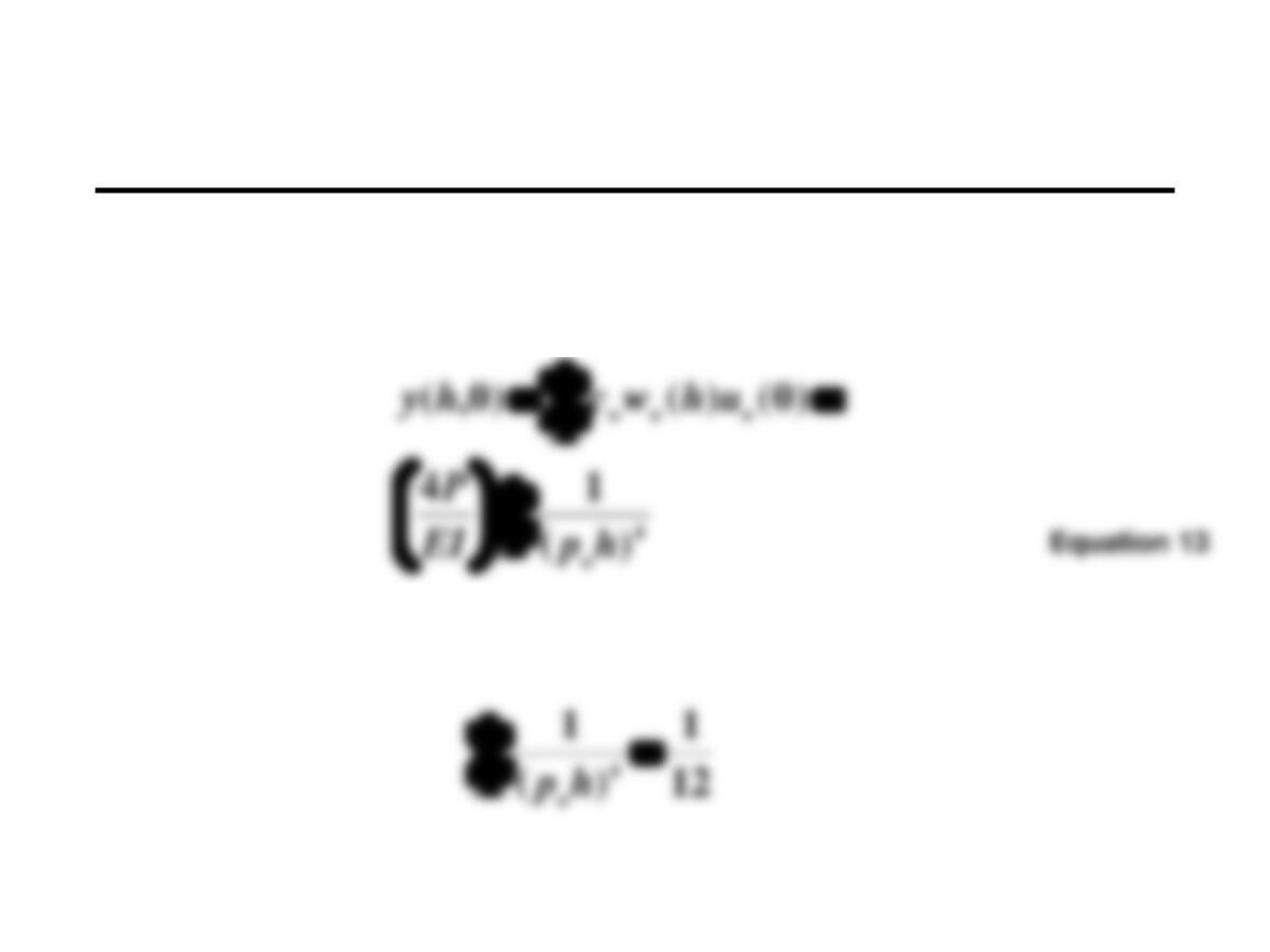
As a check on these results, we can evaluate
as given by Equations 6 through 11 at the points and
and compare to the initial condition
hx =
0=t
Analysis of Beam Motion (6)
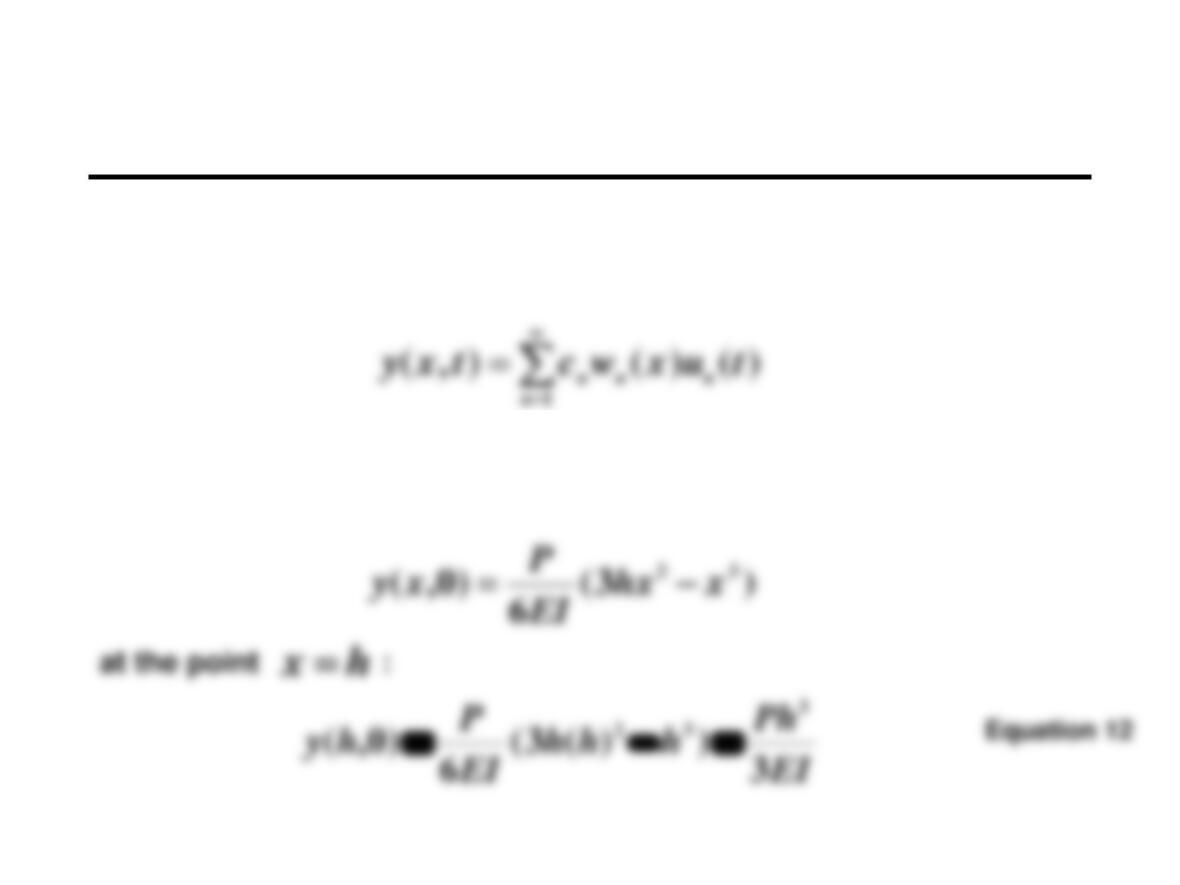
The text shows that
Comparing Equations 12 and 13 we see that we must have
Analysis of Beam Motion (7)
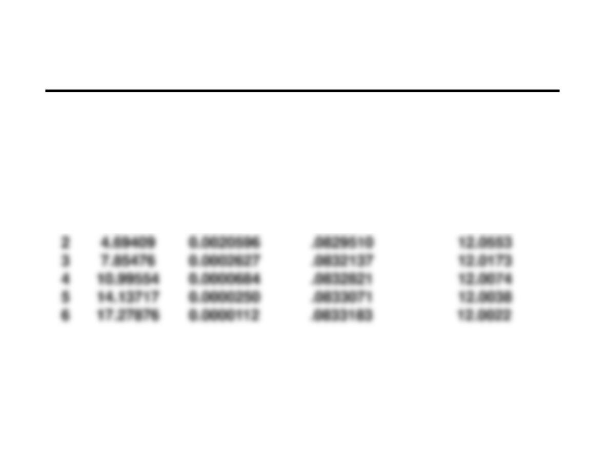
Evaluating the partial sums
The series appears to be converging to the correct result.
1 1.87510 0.0808914 .0808914 12.3623
n
hpn
4
)/(1hpn
=
n
m
mhp
1
4
)/(1
1
1
4
)/(1
−
=
n
m
mhp
Analysis of Beam Motion (8)
The text proves that the eigenfunctions satisfying the beam equation
with the given boundary conditions are orthogonal.
Furthermore (stated without proof)
There is a broad class of partial differential equations with
Beam in Resonance
The text shows how a beam excited by a cyclical input can be driven
to resonance just as an n-dimensional system can. The beam has