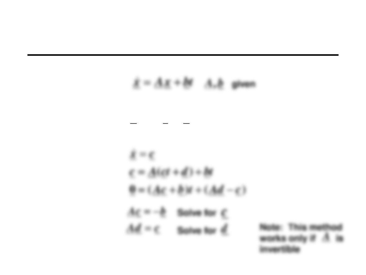
If
ttu =)(
Then try
)(
dtctx
+=
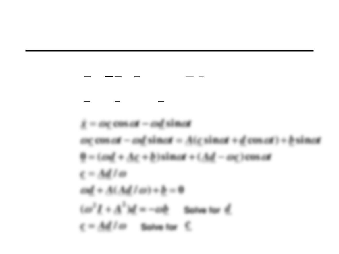
If
ttu
sin)( =
tdtctx
cossin)( +=
Then try
,, bA
given
tbxAx
sin+=
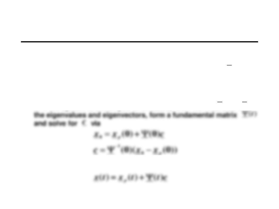
Initial Conditions
The procedure described above gives the particular solution ,
which suffices for steady state conditions with a stable and
damped system
If the solution is required to meet given initial conditions ,
or if the system is undamped or unstable, then we must also find
The full solution is then
0
)0( xx =
)(tx p

Transition to
Partial Differential Equations
Initial and Boundary Value Problems
ODEs with conditions specified only at one extreme of the independent variable
(whether it represents time or space) are called initial value problems. No
conditions are expressed at other times.
PDEs with conditions specified at the extremes of spatial coordinates over the entire
time interval are called boundary value problems.
Heat Equation
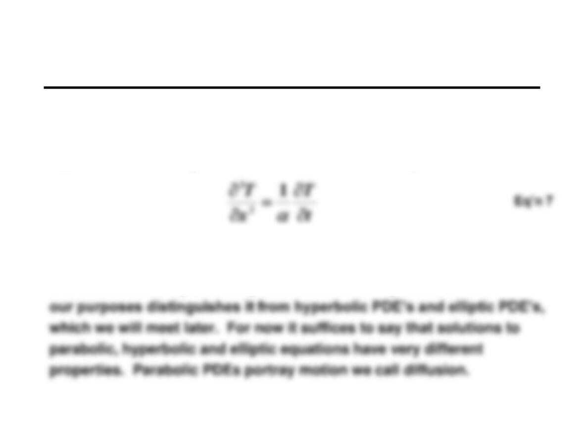
Equation 6 is the so-called heat equation, one of the fundamental
equations of the subject of heat transfer. It is usually written as
Where is called the thermal diffusivity.
It is classified as a parabolic partial differential equation, which for
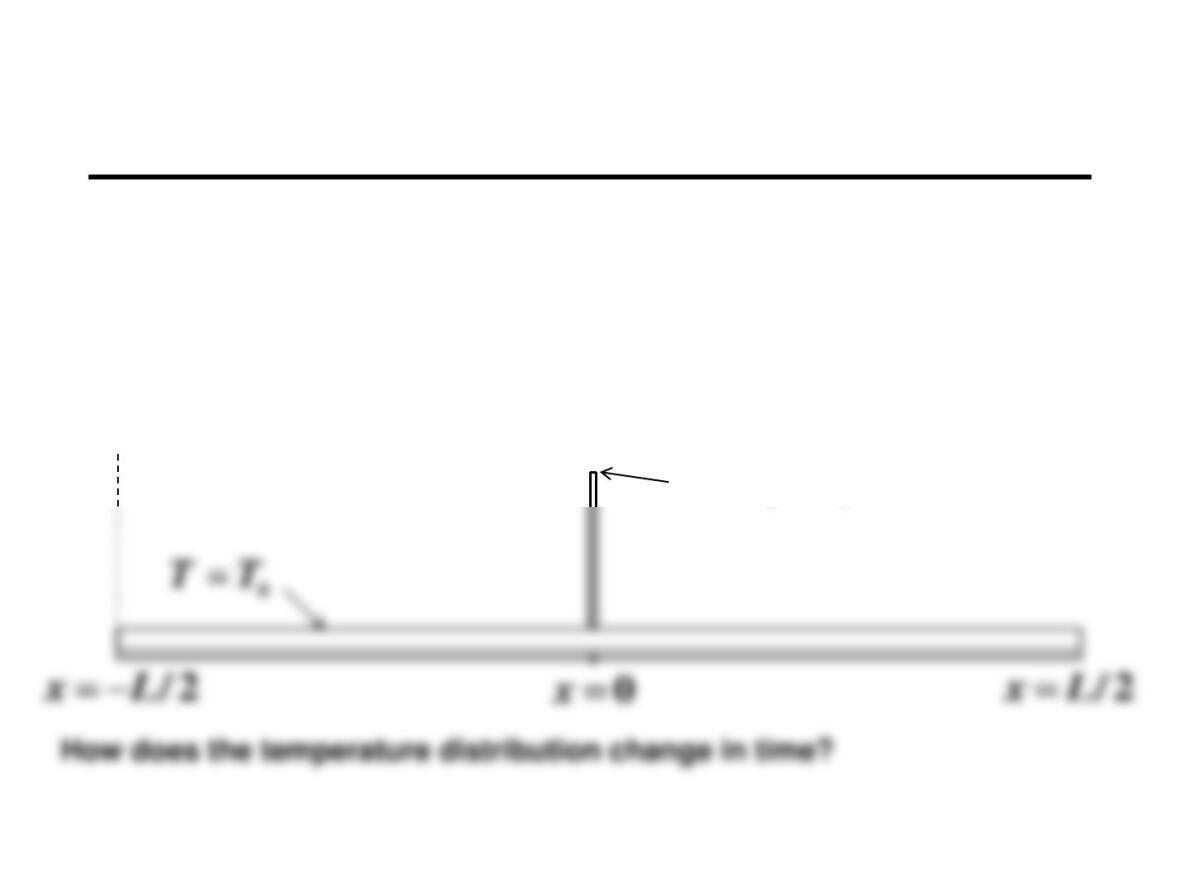
Initial Value Problem Example
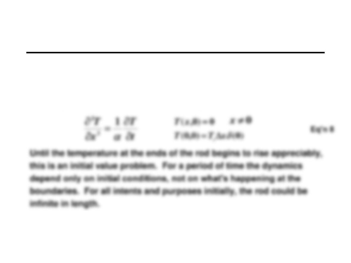
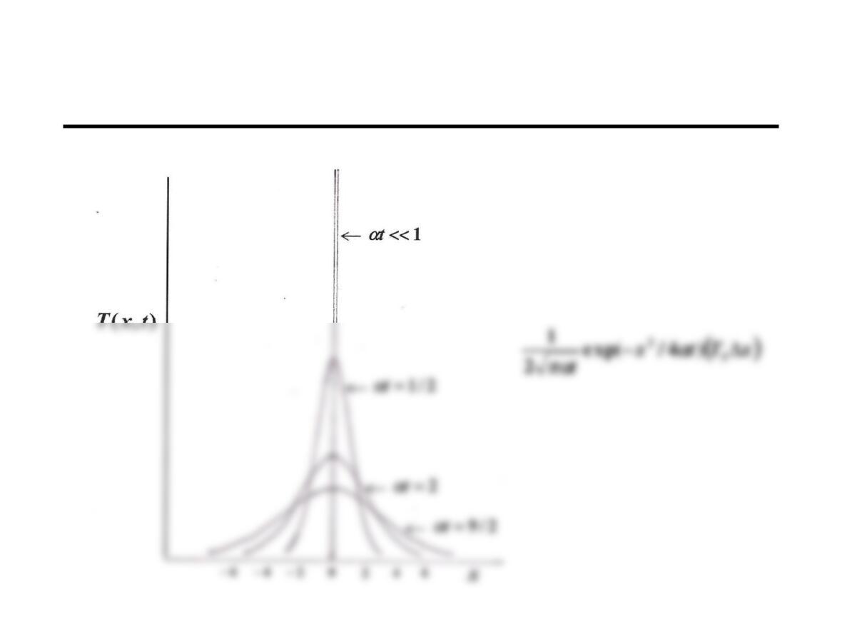
Consider a very long rod initially at a uniform temperature, to the
center of which is applied a large amount of heat in a very short time,
so that the temperature spikes in a very small region around the center
and is essentially unchanged everywhere else. At the temperature
distribution across the rod looks like this:
0=t
s
TTT += 0
x
Temperature
Initial Value Problem Example (2)
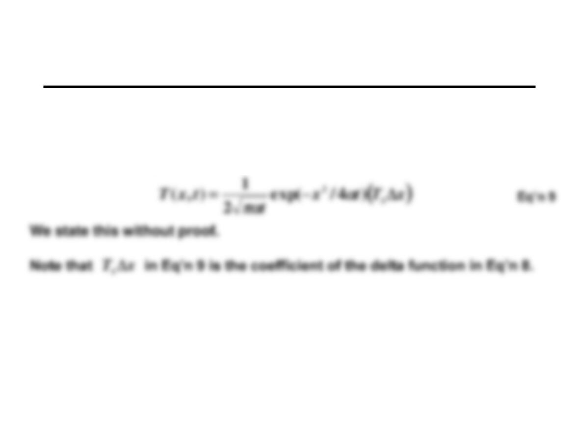
For simplicity let .
Formally, we can state the problem using the delta function:
0
0=T
Initial Value Problem Example (3)
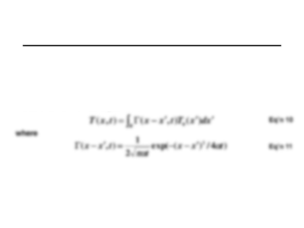
The solution to Equation 8 is
Initial Value Problem Example (4)
txT
=
),(
Initial Value Problem Example (5)
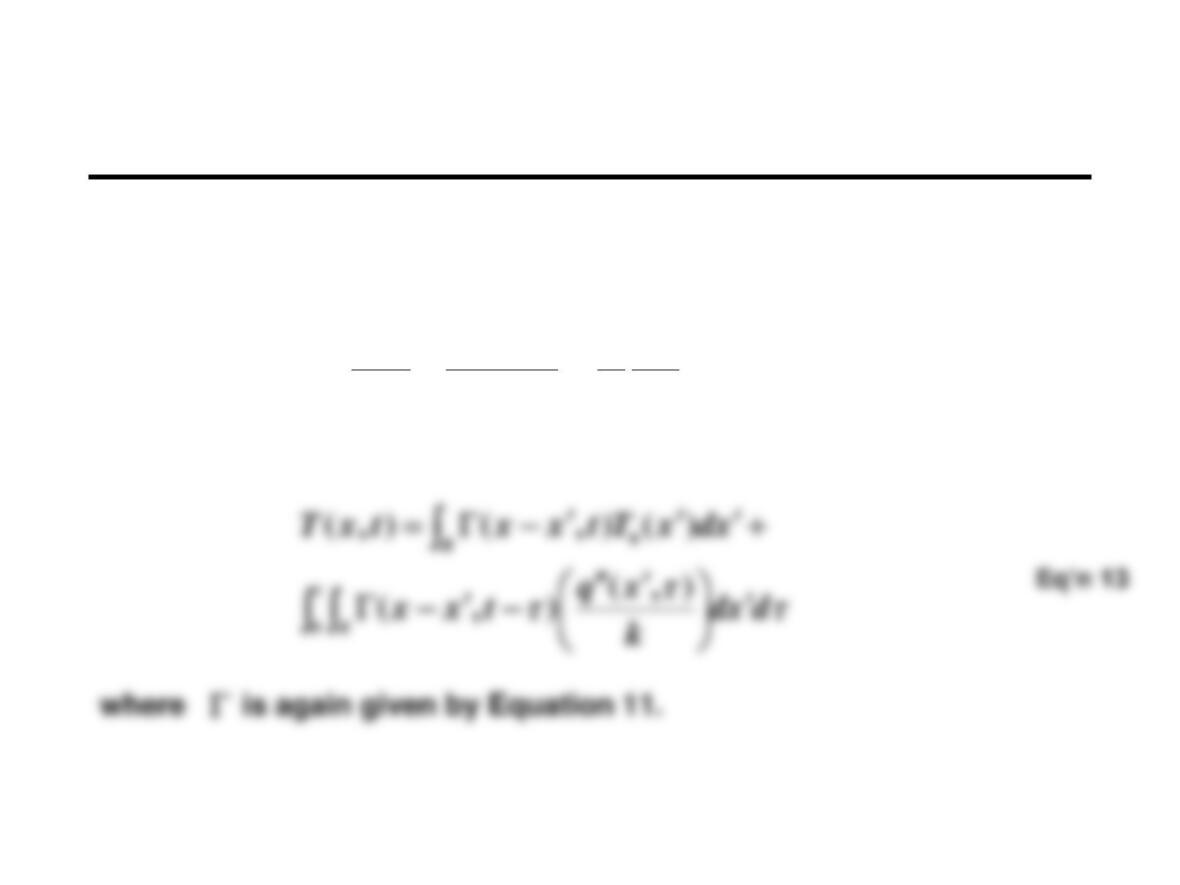
It can further be shown that for an infinite length rod and an arbitrary initial
temperature distribution
the solution to the heat equation is
)()0,( 0xTxT =
Initial Value Problem Example (6)
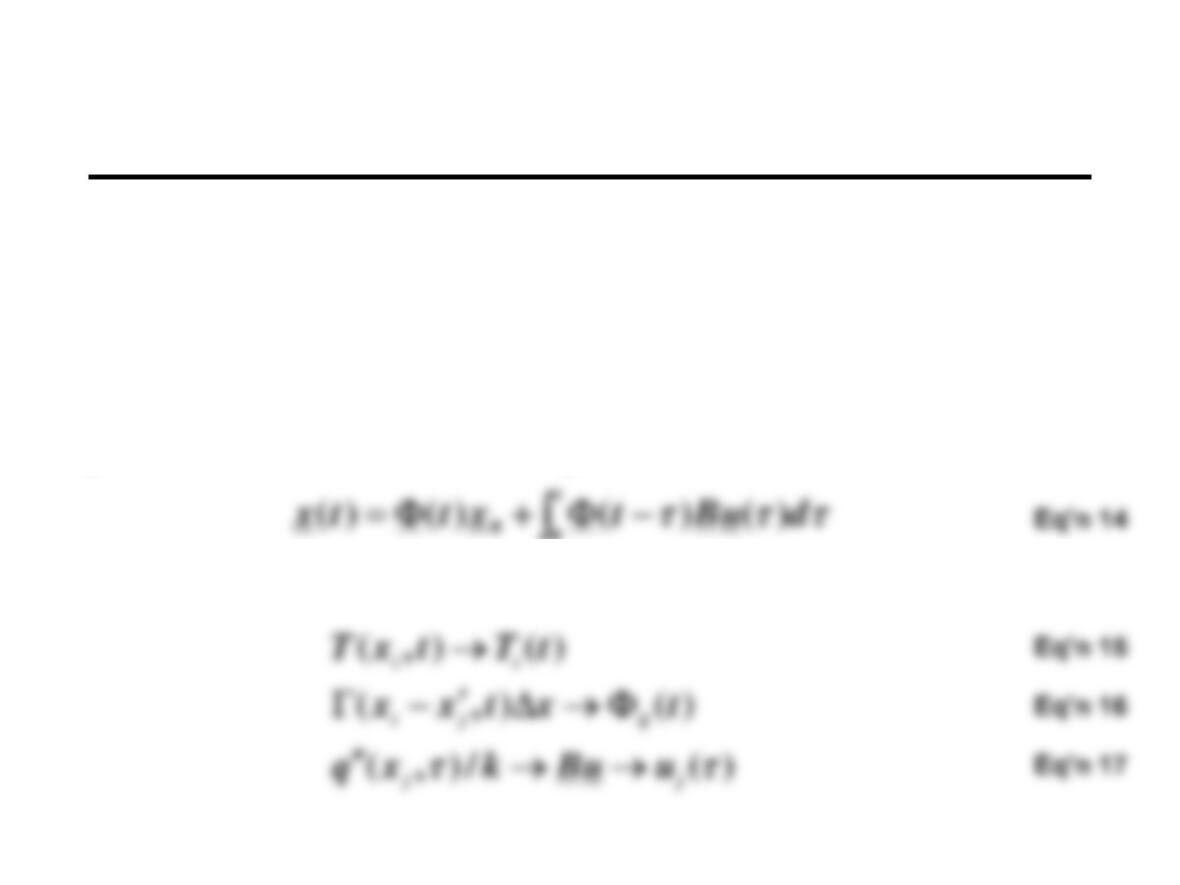
More generally yet, if there are heat sources, the heat equation is
and the solution is
t
T
k
txq
x
T
=
+
1),(
2
2
Eq’n 12
Initial Value Problem Example (7)
Equation 13 is completely analogous to solutions to initial value problems
in ordinary differential equations. The function is equivalent to the
state transition matrix.
To demonstrate the analogy, we recall the solution to linear time-invariant
systems of first order differential equations:
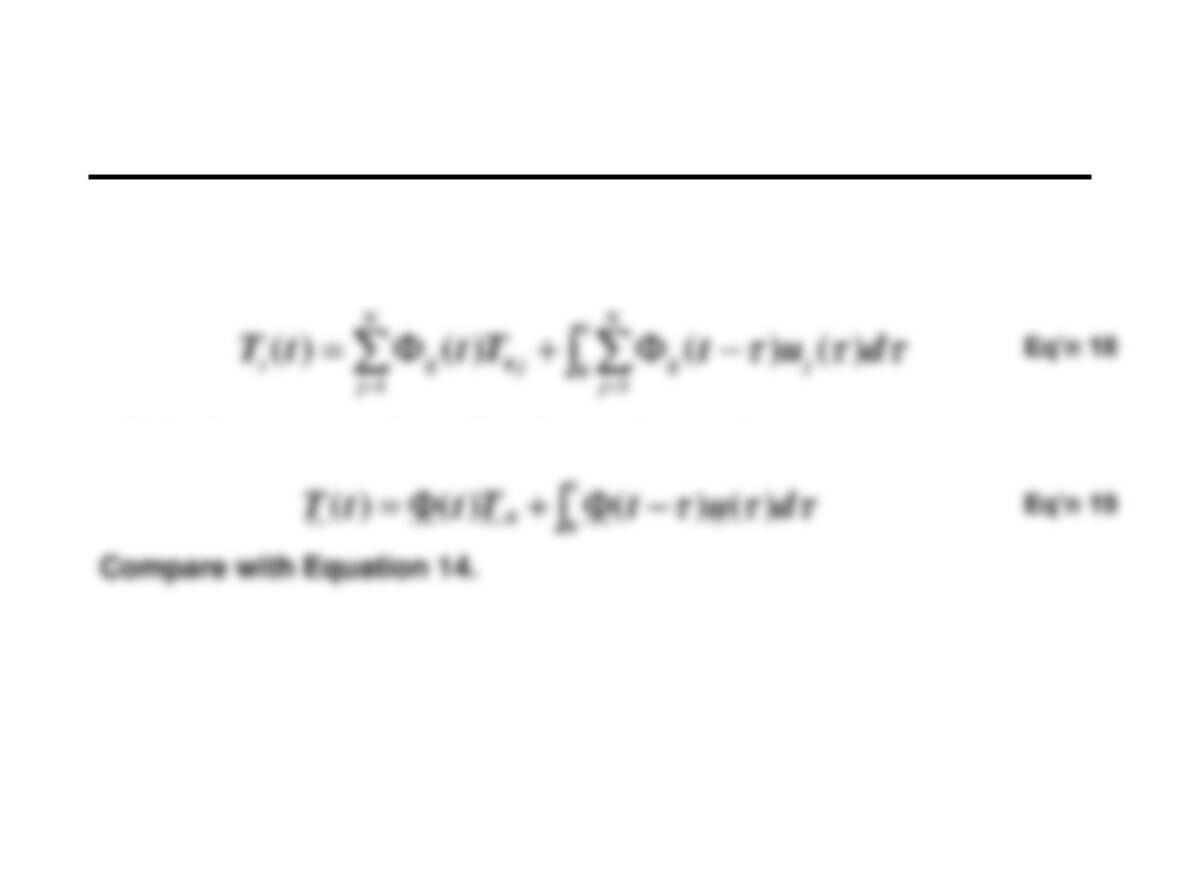
Then returning to Equation 13, we segment the rod and identify
Initial Value Problem Example (8)
Substituting Equations 15, 16 and 17 into Equation 13, we arrive at
which of course can be written in matrix notation as
In summary, the example demonstrates the strong similarity between
solutions of an important class of PDEs and those of a class of
ODEs with which we are already familiar.
Initial Value Problems:
An Existence and Uniqueness Example
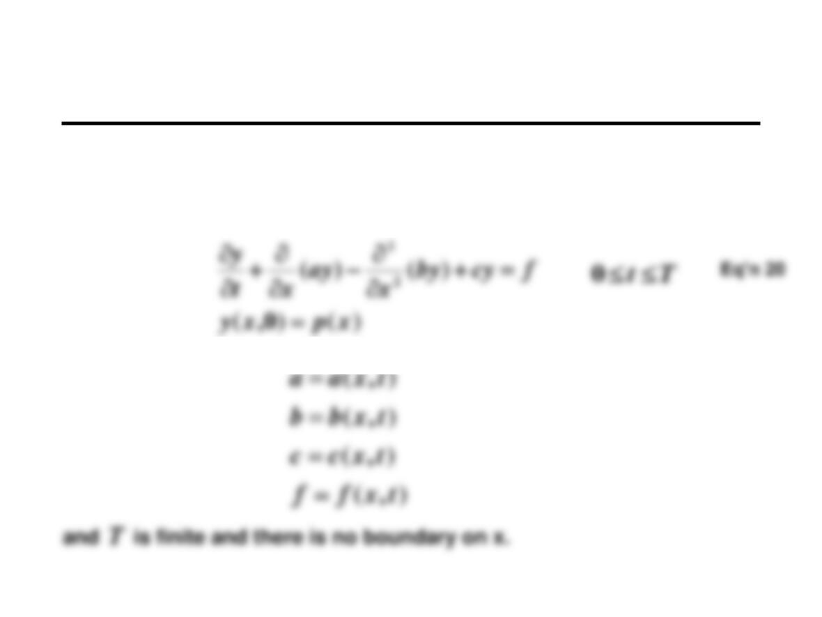
To illustrate this similarity further, consider the more general
linear parabolic PDE initial value problem described by
where
Initial Value Problems:
An Existence and Uniqueness Example (2)
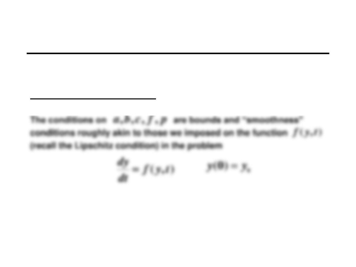
Then under certain conditions on it can be shown that
there exists a unique solution to Equation 20.
the solution of which we examined for existence and uniqueness
early in the course.
pfcba ,,,,
Homework Assignment 22
Read:
Work:
(Problems in text)