Chapter 8
Material Handling Systems Analysis
012345678
0
1
2
Revolution #1
012345678
0
1
2
Revolution #2
012345678
0
1
2
Revolution #3
012345678
0
1
2
Revolution #4
012345678
0
1
2
Revolution #5
012345678
0
1
2
Revolution #6
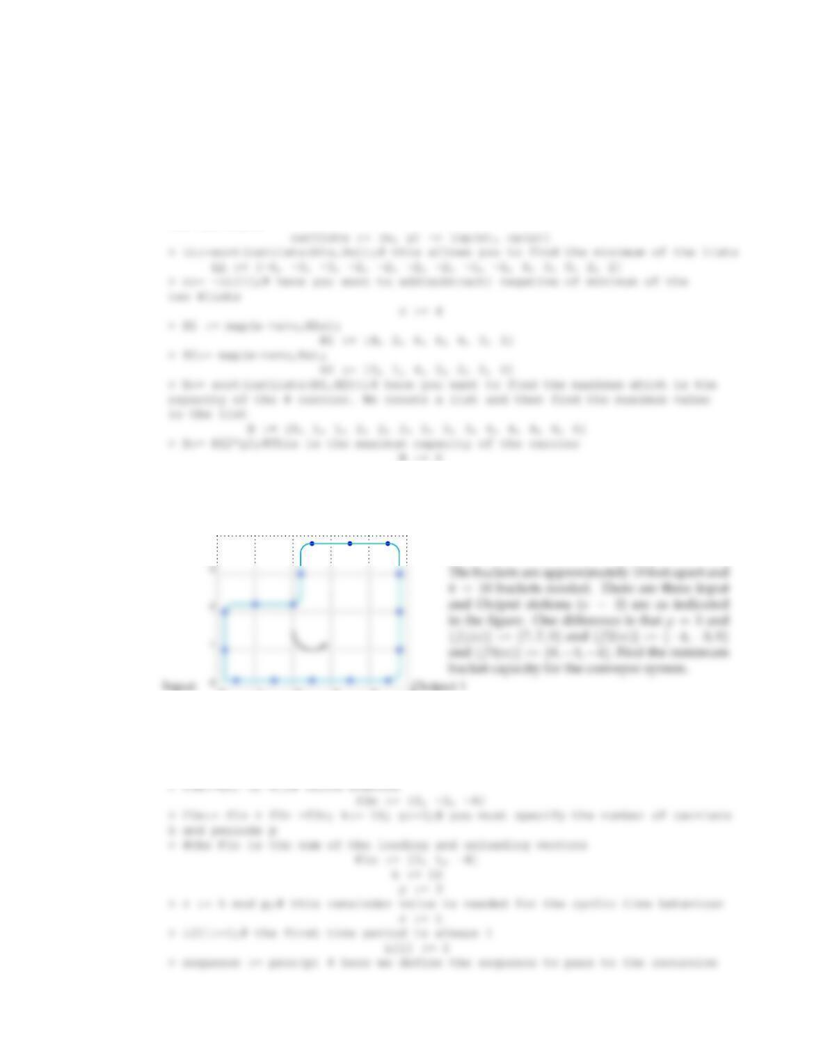
Illustration of a Closed Loop Conveyor Revolutions
10. Solutions to Exercises
1. For the Receiving area of your factory project, categorize the items for these in-bound shipments.
Estimate the time between arrivals of in-bound shipments for your factory project. Estimate the
probability distribution most appropriate for these in-bound shipments of raw materials. This is
a necessary starting point for building a dynamic model of the plant. Build an analytical model
or a simulation model of the Receiving area and correlate your estimate of the buffer and staging
(queueing) area square footage of the incoming products into Receiving area with the types of goods
incoming into the Receiving area.
1
2. For the Shipping area of your factory project, please estimate how often shipments will be made from
the plant? Also, estimate the number of docks needed for the trucks.
•This again will depend upon the overall demand for the product and the number of shipments of finished
goods they will have to made from their facility on a day-to-day basis or weekly basis. Once the students
10.. SOLUTIONS TO EXERCISES
3
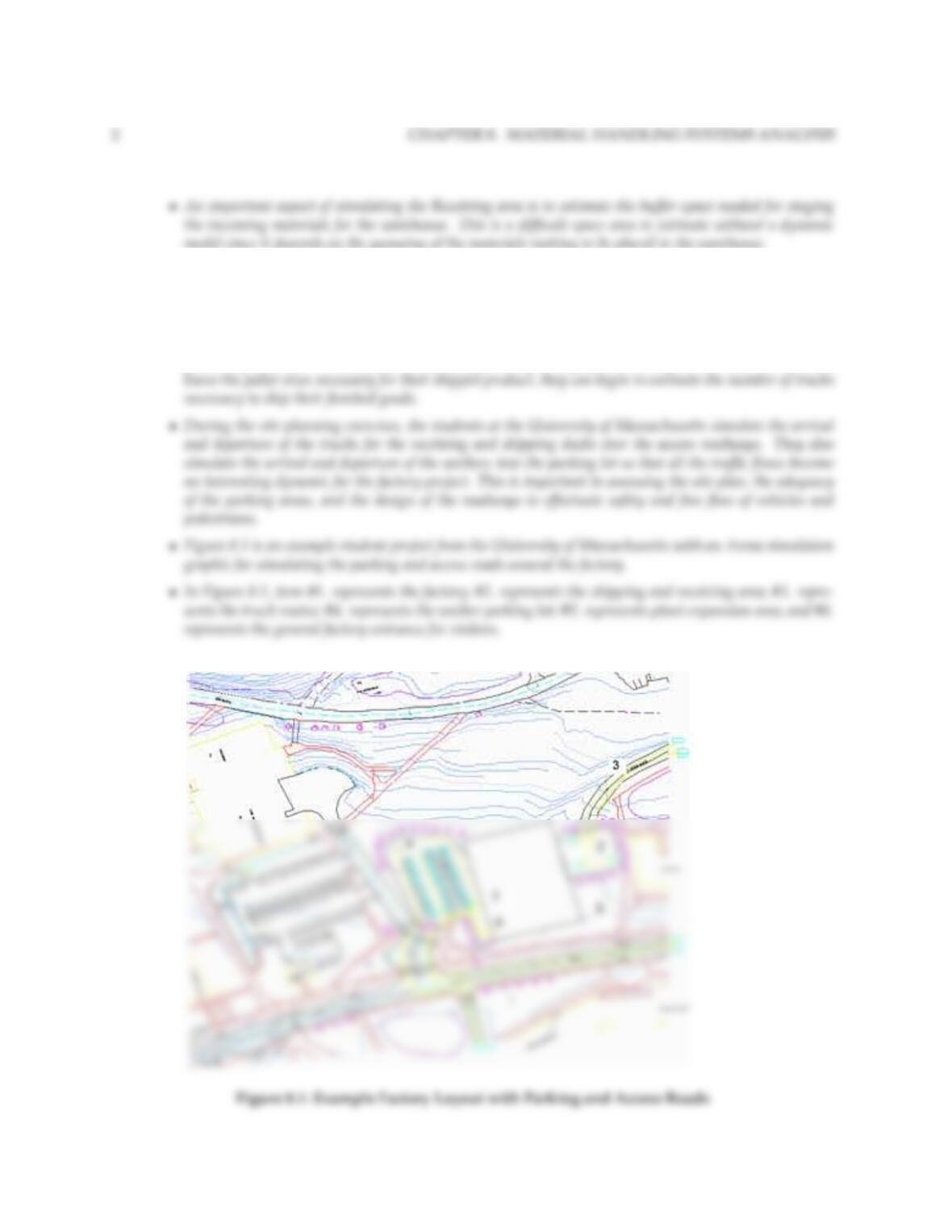
3. Take your layout as generated for the factory project and identify the material handling flow network.
Superimpose the network on the facility layout and graphically illustrate the flows throughout the
activities of the layout. With this network, argue deterministically where the queues and bottlenecks
will likely occur. Take the most significant bottleneck identified above, preferably a workstation
or subset of workstations, and either with an analytical model or a simulation model dynamically
simulate the workstation much as we did with the XYZ corporation. Compare your deterministic
estimates with the model estimates.
•Figure 8.2 illustrates the superposition of the material flow diagram on top of the factory layout for a
sample student project from the University of Massachusetts.
Figure 8.2: Example Material Handling Flow Superimposed on Factory Layout
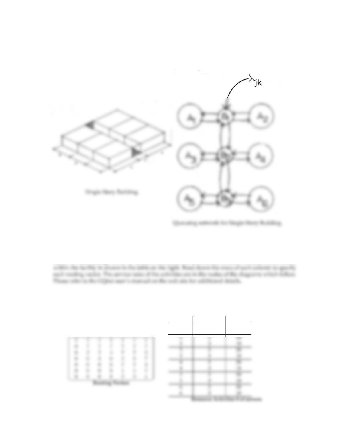
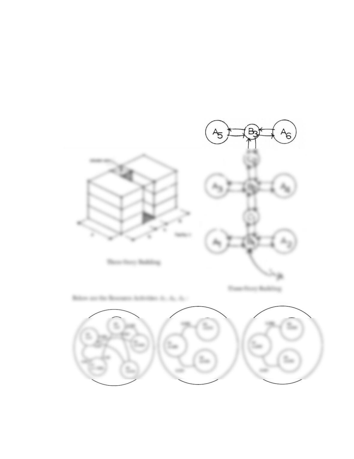
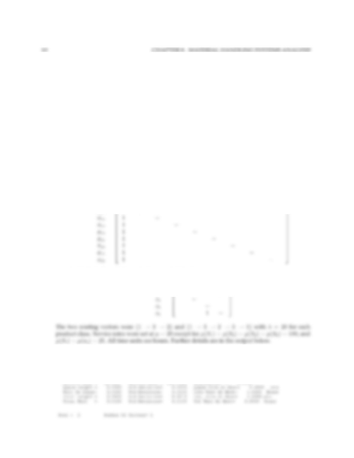
4. The figures below represent a single-story facility and its queueing network representation. Each
activity Aihas around 20 people and approximately 2400 sq.ft. B1, B2, B3represent the horizontal
circulation element adjoining the activities. This could be represented as a single node, but it allows
for more detail as three nodes. These three nodes can be modelled as M/G/∞or else as M/G/c/c
queues. We will assume seven customer classes with appropriate routing vectors and resource activ-
ities shown below.
4
CHAPTER 8. MATERIAL HANDLING SYSTEMS ANALYSIS
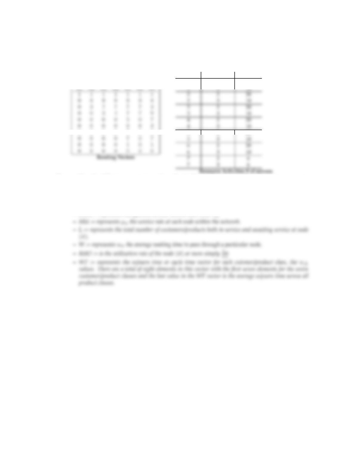
Below are the routing vectors in the first matrix on the left and the number of multi-server nodes
R1R2R3R4R5R6R7
Activity sub-activity # servers
1 2 20
1 3 10
10.. SOLUTIONS TO EXERCISES
5
#2 #4
Infor
Resource Activity A 1
#2 #4
u =6
Infor
Resource Activities A – A 6
2
Infor
Resource Activity A 7
Please utilize the GQnet program to analyze the facility and computer all performance measures
available with GQnet. Please interpret your results.
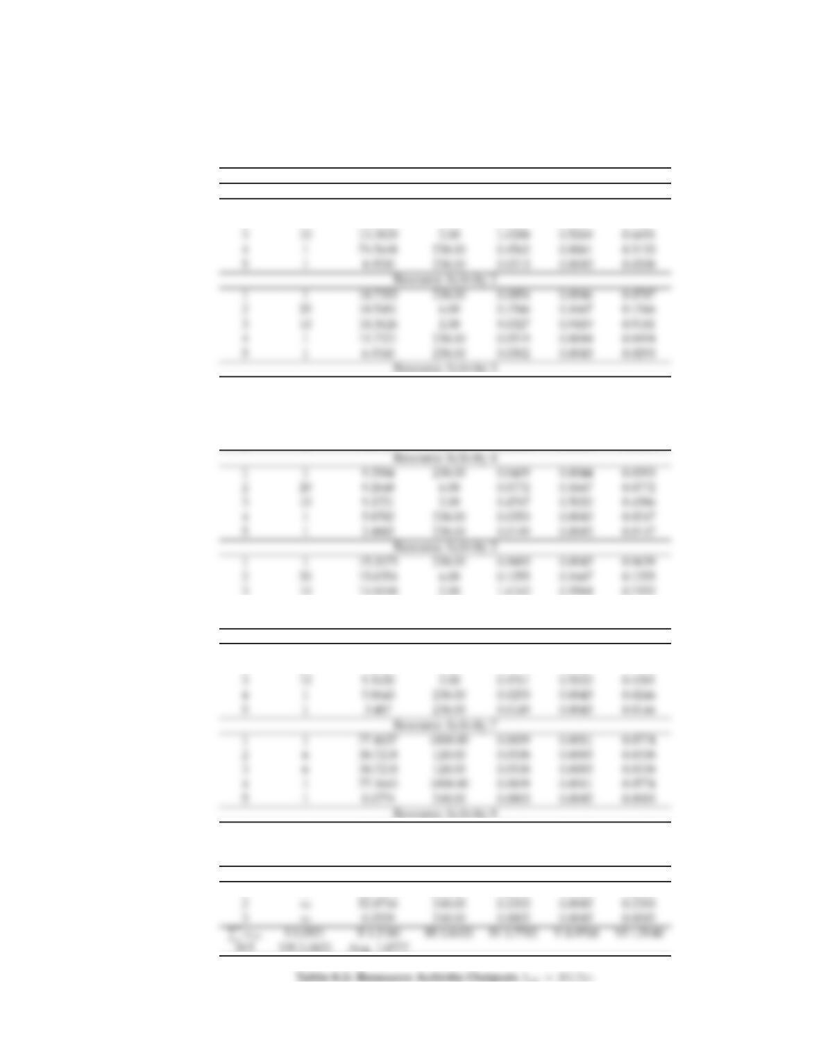
•In Table 1 is output from the Qnet computer program of the performance measures for the different
resource activities. The headings in the table are defined as follows:
–LAM := represents the effective arrival rates at each node λij
–MU := represents µit the service rate at each node within the network.
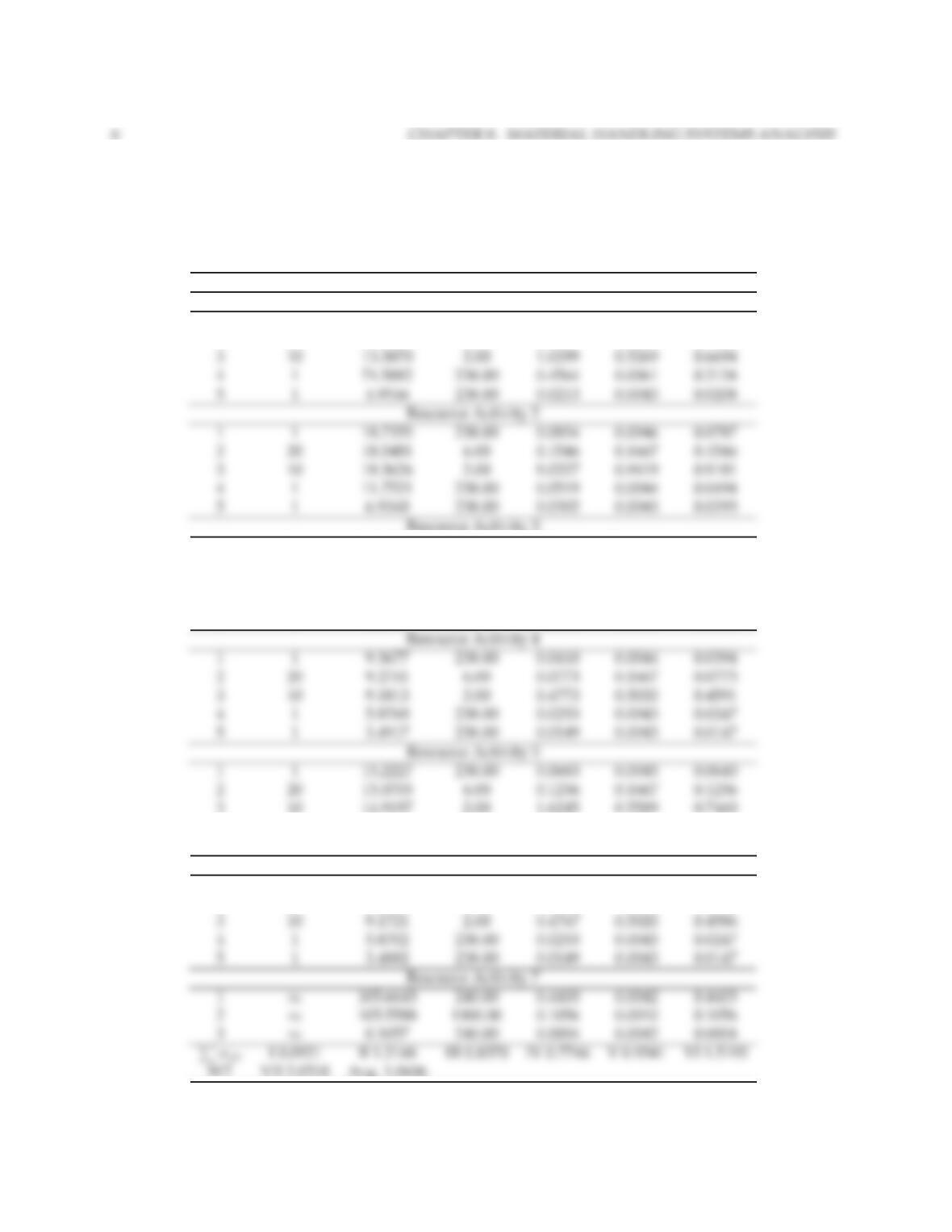
Table 8.1: Resource Activity Outputs λjk = 10/hr.
Node S LAM MU L W RHO
Resource Activity 1
1 1 79.5428 238.00 0.5020 0.0063 0.3342
2 20 13.5223 6.00 0.1127 0.1667 0.1127
1 1 15.2285 238.00 0.0684 0.0045 0.0640
2 20 15.0763 6.00 0.1256 0.1667 0.1256
3 10 14.9255 2.00 1.6277 0.5591 0.7463
4 1 9.5523 238.00 0.0418 0.0044 0.0401
5 1 5.6762 238.00 0.0244 0.0043 0.0238
4 1 9.5486 238.00 0.0418 0.0044 0.0401
5 1 5.6740 238.00 0.0244 0.0043 0.0238
Resource Activity 6
1 1 9.3584 238.00 0.0409 0.0044 0.0393
2 20 9.2648 6.00 0.0772 0.1667 0.0772
10.. SOLUTIONS TO EXERCISES
7
5. The following figures represent a three-story facility and its corresponding queueing network rep-
resentation. The B-nodes represent horizontal circulation travel and the C-nodes represent elevator
travel. In this model, we have additional resource activity nodes for the elevator, elevator waiting,
and horizontal circulation network. Resource activities A1−A6are the same as the previous problem,
whereas, activities A7, A8,and A9are as shown below. Node A7represents the elevator movement.
Node A8represents the horizontal circulation movement, and Node A9represents elevator waiting.
Resource Activity A 7
Resource Activity A 8
Resource Activity A 9
Below are the routing vectors and the number of multi-server nodes within the facility. Notice that
the elevator waiting A9precedes the elevator movement A7. Two A7nodes in succession represent
movement between two floors.
8
CHAPTER 8. MATERIAL HANDLING SYSTEMS ANALYSIS
0000759
Activity sub-activity # servers
1 2 20
5 2 20
Please utilize the GQnet program to analyze the facility and computer all performance measures
available with GQnet.
•On the next page is output from the Qnet computer program of the performance measures for the different
resource activities. The headings in the table are defined as follows:
–LAM := represents the effective arrival rates at each node λij
10.. SOLUTIONS TO EXERCISES
9
Node S LAM MU L W RHO
Resource Activity 1
1 1 79.5178 238.00 0.5017 0.0063 0.3341
2 20 13.5180 6.00 0.1127 0.1667 0.1127
1 1 15.2277 238.00 0.0683 0.0045 0.0640
2 20 15.0705 6.00 0.1256 0.1667 0.1256
3 10 14.9197 2.00 1.6245 0.5589 0.7460
4 1 9.5486 238.00 0.0418 0.0044 0.0401
5 1 5.6740 238.00 0.0244 0.0043 0.0238
4 1 9.5391 238.00 0.0418 0.0044 0.0401
5 1 5.6684 238.00 0.0244 0.0043 0.0238
Resource Activity 6
1 1 9.340 238.00 0.0409 0.0044 0.0393
2 20 9.2555 6.00 0.0771 0.1667 0.0771
1∞24.6185 240.00 0.1026 0.0042 0.1026
2∞24.5939 240.00 0.1025 0.0042 0.1025
3∞0.0246 240.00 0.0001 0.0042 0.0001
Resource Activity 9
1∞52.9273 240.00 0.2205 0.0042 0.2205
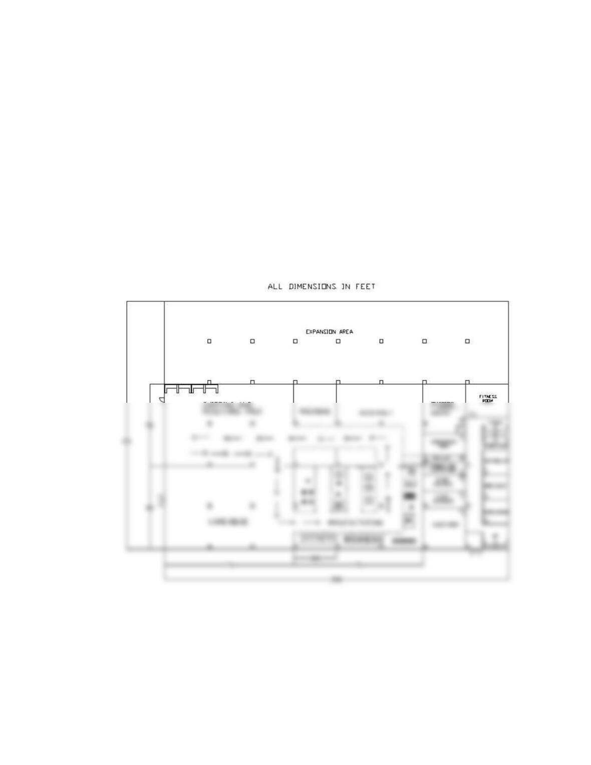
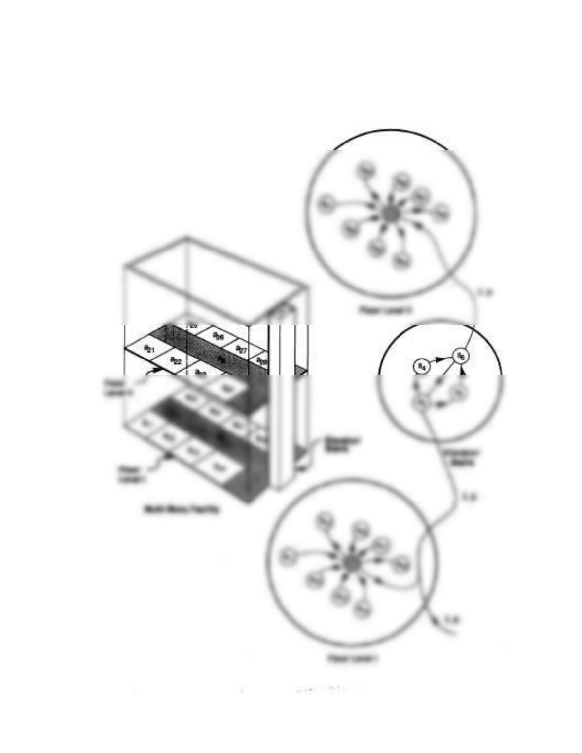
6. Figure 8.3 is an illustration of another two-story office facility. Please estimate the number of cus-
tomer classes λjk arriving at the facility along with their length of route and the activities they will
be visiting. You can vary the number of generating sources as well as the number of classes within
each generating source.
Detail the Resource Activities Aij ,∀(i, j)on the two floors as necessary. You be the judge with regard
to the amount of detail. You might start out small with the number of sub-activities, then proceed to
increase their number. A series of experiments might be in order.
Nodes S1and S2are the corridor circulation areas whereas S4is elevator travel and S5is stairwell
travel whereas S3and S6are landing areas on the two floors. S1and S2can be modelled as M/G/∞
or else as M/G/c/c queues. See the user manual for further details. Run the model GQnet by varying
the arrival rate of the customer classes and identify the key bottlenecks of your system as λjk varies.
•Floor Level I will be treated as a Resource Activity A1and so will floor level two as A2. The vertical
travel will also be treated as a Resource Activity A3. There is currently a limit of nine sub-activities for
each resource activity due to a program limitation. For each floor level I and II, the following transition
matrix is utilized in the Resource Activity description, which represents a star network topology.
activities S1B11 B12 B13 B14 B15 B16 B17 B18
S1−0.125 0.125 0.125 0.125 0.125 0.125 0.125 0.125
B11 1−
For the Vertical circulation node, Resource Activity A3
activities S3S4S5S6
S3−0.95 0.05
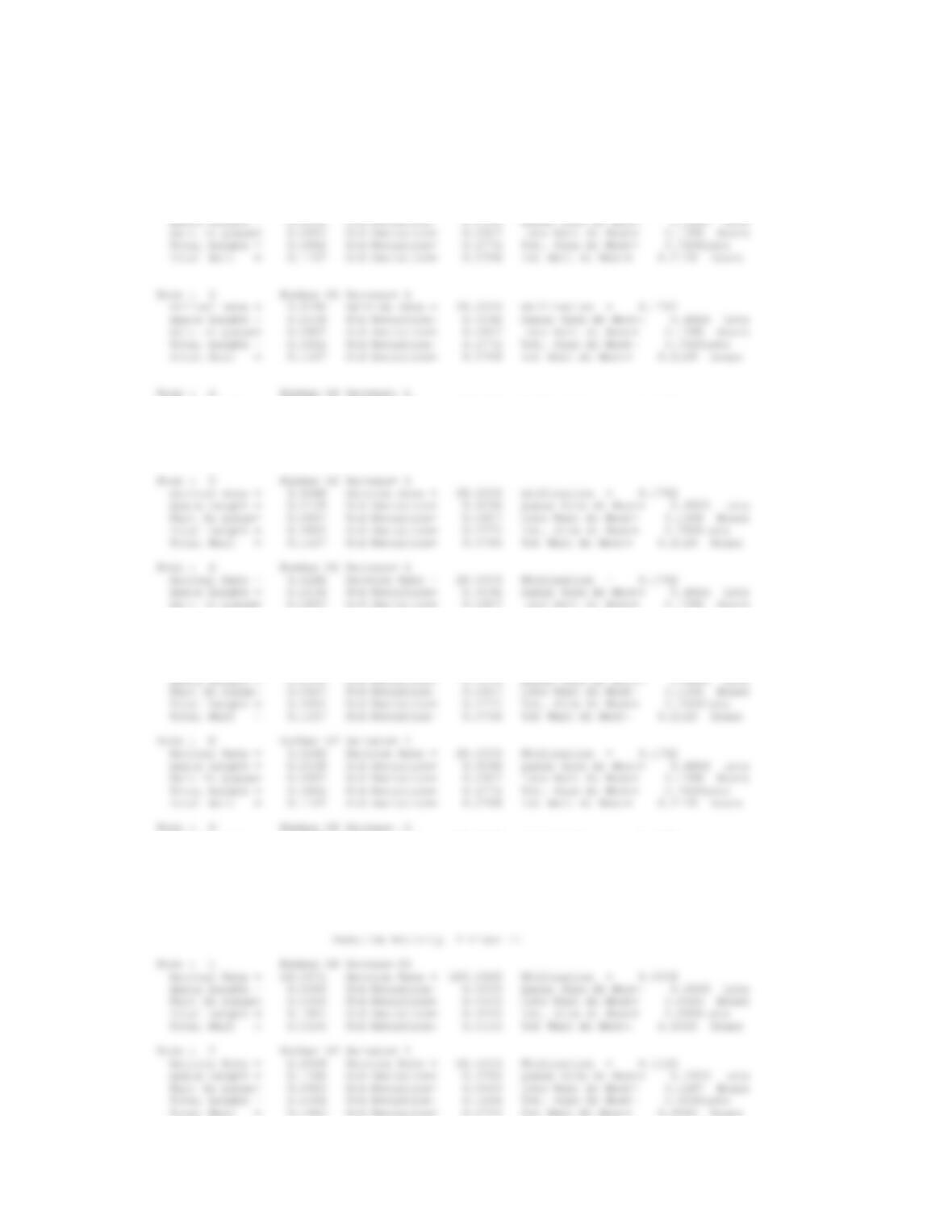
The results from GQnet appear below.
Resource Activity 1 Floor I
Node : 1 Number Of Servers=99
10.. SOLUTIONS TO EXERCISES
11
Figure 8.3: Two-story Office Facility
12
CHAPTER 8. MATERIAL HANDLING SYSTEMS ANALYSIS
Arrival Rate = 3.5246 Service Rate = 20.0000 Utilization = 0.1762
Arrival Rate = 3.5246 Service Rate = 20.0000 Utilization = 0.1762
Queue Length = 0.2139 Std Deviation= 0.5096 Queue Size At Most= 0.4926 Lots
Wait In Queue= 0.0607 Std Deviation= 0.0607 Lots Wait At Most= 0.1398 Hours
Total Length = 0.3902 Std Deviation= 0.2772 Tot. Size At Most= 0.7505Lots
Total Wait = 0.1107 Std Deviation= 0.0786 Tot Wait At Most= 0.2129 Hours
Total Length = 0.3902 Std Deviation= 0.2772 Tot. Size At Most= 0.7505Lots
Total Wait = 0.1107 Std Deviation= 0.0786 Tot Wait At Most= 0.2129 Hours
Node : 7 Number Of Servers= 1
Arrival Rate = 3.5246 Service Rate = 20.0000 Utilization = 0.1762
Arrival Rate = 3.5246 Service Rate = 20.0000 Utilization = 0.1762
Queue Length = 0.2139 Std Deviation= 0.5096 Queue Size At Most= 0.4926 Lots
Wait In Queue= 0.0607 Std Deviation= 0.0607 Lots Wait At Most= 0.1398 Hours
Total Length = 0.3902 Std Deviation= 0.2772 Tot. Size At Most= 0.7505Lots
Total Wait = 0.1107 Std Deviation= 0.0786 Tot Wait At Most= 0.2129 Hours
10.. SOLUTIONS TO EXERCISES
13
Node : 3 Number Of Servers= 1
Arrival Rate = 2.2509 Service Rate = 20.0000 Utilization = 0.1125
Queue Length = 0.1268 Std Deviation= 0.3780 Queue Size At Most= 0.2920 Lots
Queue Length = 0.1268 Std Deviation= 0.3780 Queue Size At Most= 0.2920 Lots
Wait In Queue= 0.0563 Std Deviation= 0.0563 Lots Wait At Most= 0.1297 Hours
Total Length = 0.2394 Std Deviation= 0.1696 Tot. Size At Most= 0.4598Lots
Total Wait = 0.1063 Std Deviation= 0.0753 Tot Wait At Most= 0.2043 Hours
Total Wait = 0.1063 Std Deviation= 0.0753 Tot Wait At Most= 0.2043 Hours
Node : 8 Number Of Servers= 1
Arrival Rate = 2.2509 Service Rate = 20.0000 Utilization = 0.1125
Queue Length = 0.1268 Std Deviation= 0.3780 Queue Size At Most= 0.2920 Lots
Arrival Rate = 28.5716 Service Rate = 100.0000 Utilization = 0.2857
Queue Length = 0.4000 Std Deviation= 0.7483 Queue Size At Most= 0.9210 Lots
Wait In Queue= 0.0140 Std Deviation= 0.0140 Lots Wait At Most= 0.0322 Hours
Total Length = 0.6857 Std Deviation= 0.4916 Tot. Size At Most= 1.3248Lots
Total Wait = 0.0240 Std Deviation= 0.0172 Tot Wait At Most= 0.0464 Hours
Wait In Queue= 0.0424 Std Deviation= 0.0424 Lots Wait At Most= 0.0977 Hours
Total Length = 0.1177 Std Deviation= 0.0833 Tot. Size At Most= 0.2260Lots
Total Wait = 0.0824 Std Deviation= 0.0583 Tot Wait At Most= 0.1582 Hours
Node : 4 Number Of Servers=99
7. A closed-loop conveyor has seven equally-spaced carriers and two stations, one input and one output
station.
s= 2, k = 7, p = 5, r = 7 mod 5 = 2
Loading Station {f1(n)}:= {0,0,3,2,1}
Unloading Station {f2(n)}:= {0,0,0,−2,−4}
b) Find the minimum bucket size for different numbers of carriers k= 6,…9.
f1n:=[0,0,3,2,1];# here are the loading values
f1n := [0, 0, 3, 2, 1]
> f2n:=[0,0,0,-2,-4];# here are the unloading values
10.. SOLUTIONS TO EXERCISES
15
> end do:
> end proc:
> sequence(p);
> print(L);
> kwo1(L,p);
[0, 0, 3, 3, 0]
> c:= -LL[1];# here you want to add(subtract) negative of minimum
of the two #lists
c := 1
> H1 := map(x->x+c,H1s);
H1 := [1, 1, 4, 4, 1]
> H2:= map(x->x+c,Hs);
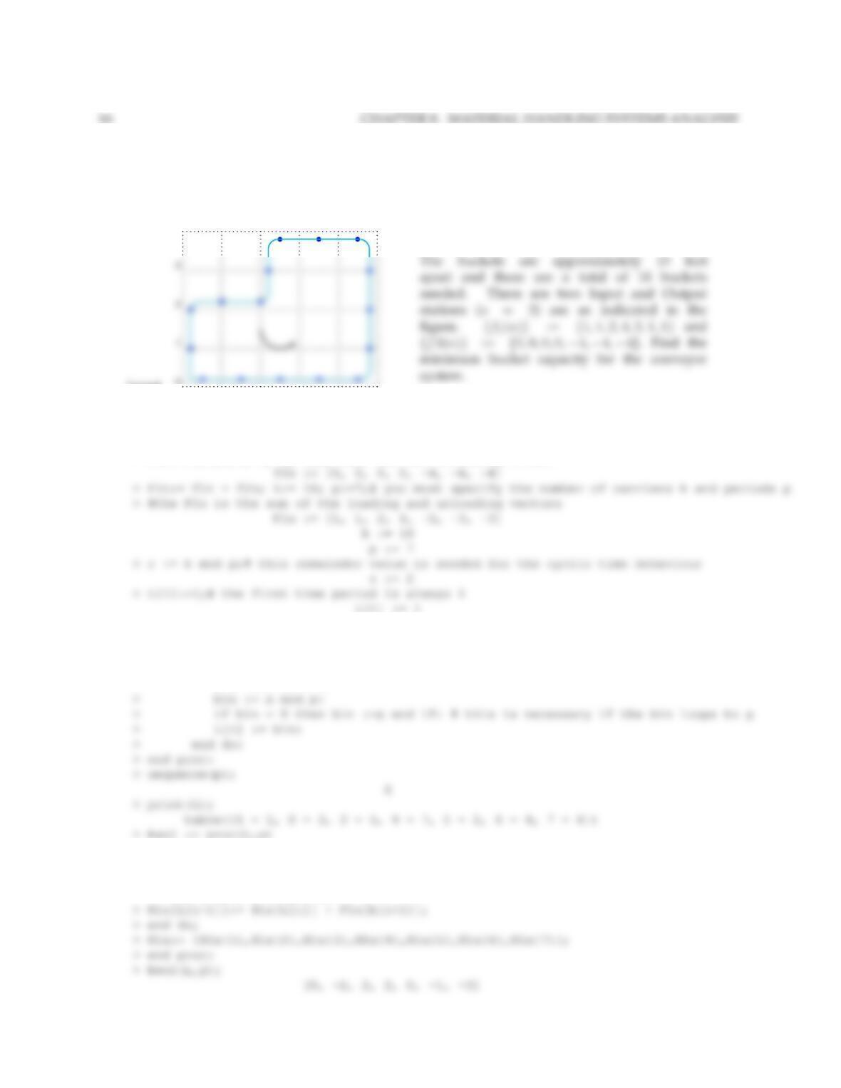
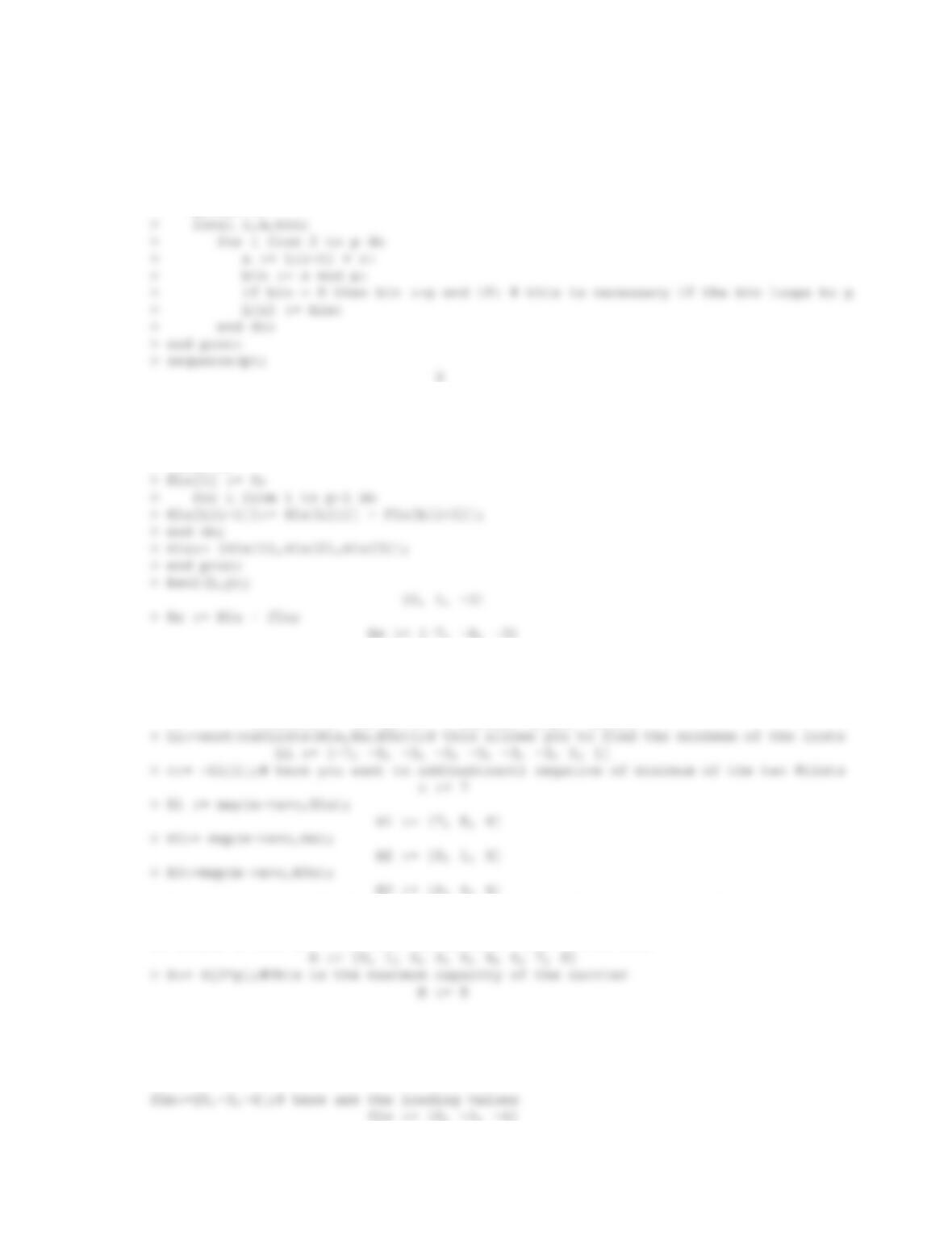
8. You are designing a layout with an overhead bucket conveyor connecting the following portions of
an assembly area within a plant.
0 1 2 3 4 5
4
Input
Output
f1n:=[1,1,2,4,2,1,1];# here are the loading values
f1n := [1, 1, 2, 4, 2, 1, 1]
> f2n:=[0,0,0,0,-4,-4,-4];# here are the unloading values
> sequence := proc(p) # here we define the sequence to pass to the recursion
> global L;
> local i,x,bin;
> for i from 2 to p do
> x := L[i-1] + r:
> global H1s;
> local i;
> H1s[1] := 0;
> for i from 1 to p-1 do
10.. SOLUTIONS TO EXERCISES
17
> Hs := H1s – f1n;
Hs := [-1, -3, 0, -2, -2, -2, -4]
> catLists:= (x,y)->[op(x),op(y)];# here you define a function to concatenate
the two lists
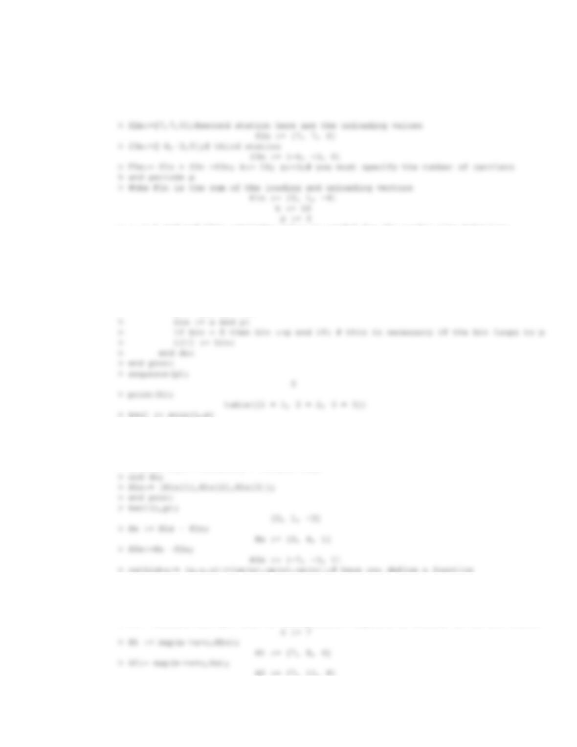
9. Now let’s say that you are re-designing the previous layout with an overhead bucket conveyor and
you are adding another output station to the assembly area within a plant.
0 1 2 3 4 5
4
Output 2
> f1n:=[7,7,0];# here are the loading values
f1n := [7, 7, 0]
> f2n:=[-4,-3,0];#second station here are the unloading values
f2n := [-4, -3, 0]
18
CHAPTER 8. MATERIAL HANDLING SYSTEMS ANALYSIS
> global L;
> print(L);
table([1 = 1, 2 = 2, 3 = 3])
> kwo1 := proc(L,p)
> global H1s;
> local i;
> H3s:=Hs -f2n;
H3s := [-3, -3, -3]
> catLists:= (x,y,z)->[op(x),op(y),op(z)];# here you define a function to
concatenate the two lists
catLists := (x, y, z) -> [op(x), op(y), op(z)]
> B:= sort(catLists(H1,H2,H3));# here you want to find the maximum which is the
capacity of the # carrier.
We create a list and then find the maximum value in the list
10. Also, as another variation on the last problem, say that you can reposition the input station, so
that the loading and unloading patterns are shifted, so that {f1(n)}:= {0,−3,−4}and {f2(n)}:=
{7,7,0}and {f3(n)}:= {−4,−3,0}.What is the new bucket capacity?
10.. SOLUTIONS TO EXERCISES
19
> r := k mod p;# this remainder value is needed for the cyclic time behaviour
r := 1
> L[1]:=1;# the first time period is always 1
L[1] := 1
> sequence := proc(p) # here we define the sequence to pass to the recursion
> global L;
> local i,x,bin;
> for i from 2 to p do
> x := L[i-1] + r:
> global H1s;
> local i;
> H1s[1] := 0;
> for i from 1 to p-1 do
> H1s[L[i+1]]:= H1s[L[i]] + F1n[L[i+1]];
to concatenate the two lists
catLists := (x, y, z) -> [op(x), op(y), op(z)]
> LL:=sort(catLists(H1s,Hs,H3s));# this allows you to find the minimum of the lists
LL := [-7, -3, -3, 0, 0, 1, 1, 1, 4]
> c:= -LL[1];# here you want to add(subtract) negative of minimum of the two #lists
11. Create a model with the GQnet program that represents a system or subsystem of the factory project
and run it with the GQnet program. Be sure to identify the product classes, routing vectors, service
rates, and numbers of servers required according to the program requirements.
12. Create a series, merge and or splitting system based upon your factory project and analyze it with
the closed queueing network model. The assembly system of your product is a good area of the
plant to focus on, since you will most likely have conveyors with finite buffers. If you have access
to a simulation program, compare the closed queueing network model with the simulation model.
Be sure to properly put the buffers in the system that the optimization routine outputs of the closed
queueing network model for your project system configuration.