Applied Statistics and Probability for Engineers, 7th edition 2017
8-1
CHAPTER 8
Section 8.1
8.1.1 a) The confidence level for
2.14 / 2.14 /x n x n
− +
8.1.2 a) A z = 1.29 would result in a 90% one-sided confidence interval.
8.1.3 a) Sample mean from the first confidence interval = 38.02 + (61.98 − 38.02)/2 = 50.
8.1.5 a) The 99% CI on the mean calcium concentration would be wider.
8.1.6 95% Two-sided CI on the true mean yield: where
x
= 90.480,
= 3, n = 5 and z0.025 = 1.96.
Applied Statistics and Probability for Engineers, 7th edition 2017
8-2
8.1.7 a) 99% Two-sided CI on the true mean piston ring diameter
8.1.8 a) 95% two sided CI on the mean compressive strength
8.1.9 99% confidence that the error of estimating the true compressive strength is less than 15 psi.
Applied Statistics and Probability for Engineers, 7th edition 2017
8-3
8.1.10 If n is doubled in equation 8-7:
/2 /2
x z x z
nn
− +
8.1.11 To decrease the length of the CI by one half, the sample size must be increased by 4 times (22).
8.1.12 a) 95% CI for μ, n = 5
= 0.66
3.372,x=
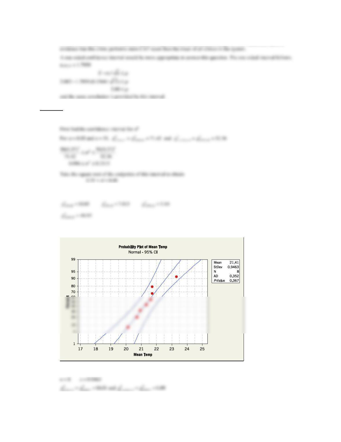
8.1.13 a) 99% two sided CI on the mean temperature
b) 95% lower-confidence bound on the mean temperature.
Applied Statistics and Probability for Engineers, 7th edition 2017
8-4
c) 95% confidence that the error of estimating the mean temperature for wheat grown is less than
2 degrees Celsius.
d) Set the width to 1.5 degrees Celsius with
= 0.5, z0.025 = 1.96 solve for n.
Section 8.2
8.2.1 a)
sum 251.848 25.1848
1
Mean 0N
= = =
8.2.2 For 1-tailed t-tests:
8.2.3 95% confidence interval on mean tire life
8.2.6 95% confidence interval on mean peak power
Applied Statistics and Probability for Engineers, 7th edition 2017
8-5
8.2.7
0.005,9
10 317.2 15.7 3.250n x s t= = = =
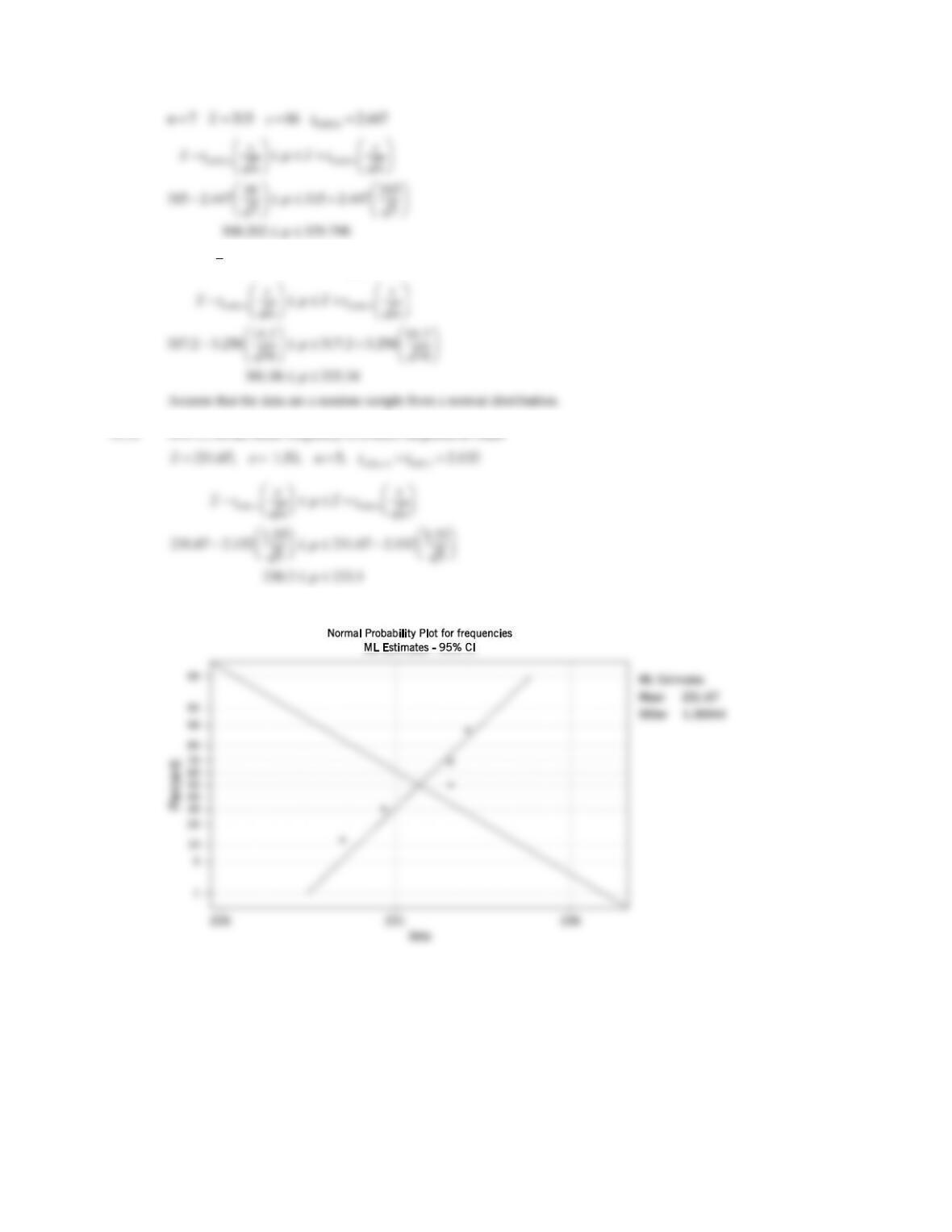
8.2.8 90% CI on the mean frequency of a beam subjected to loads
By examining the normal probability plot, it appears that the data are normally distributed.
Applied Statistics and Probability for Engineers, 7th edition 2017
8-6
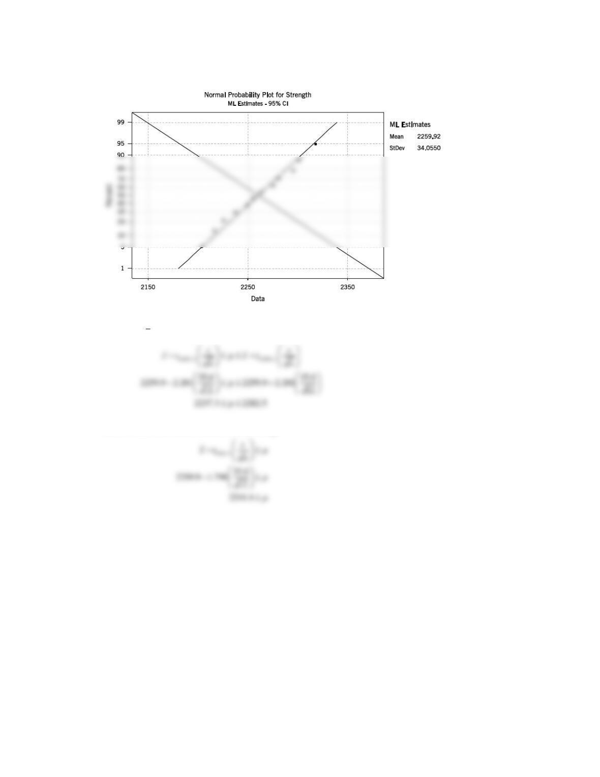
8.2.9 a) The data appear to be normally distributed based on examination of the normal probability plot below.
b) 95% two-sided confidence interval on mean comprehensive strength
0.025,11
12 2259.9 35.6 2.201n x s t= = = =
c) 95% lower-confidence bound on mean strength
Applied Statistics and Probability for Engineers, 7th edition 2017
8-7
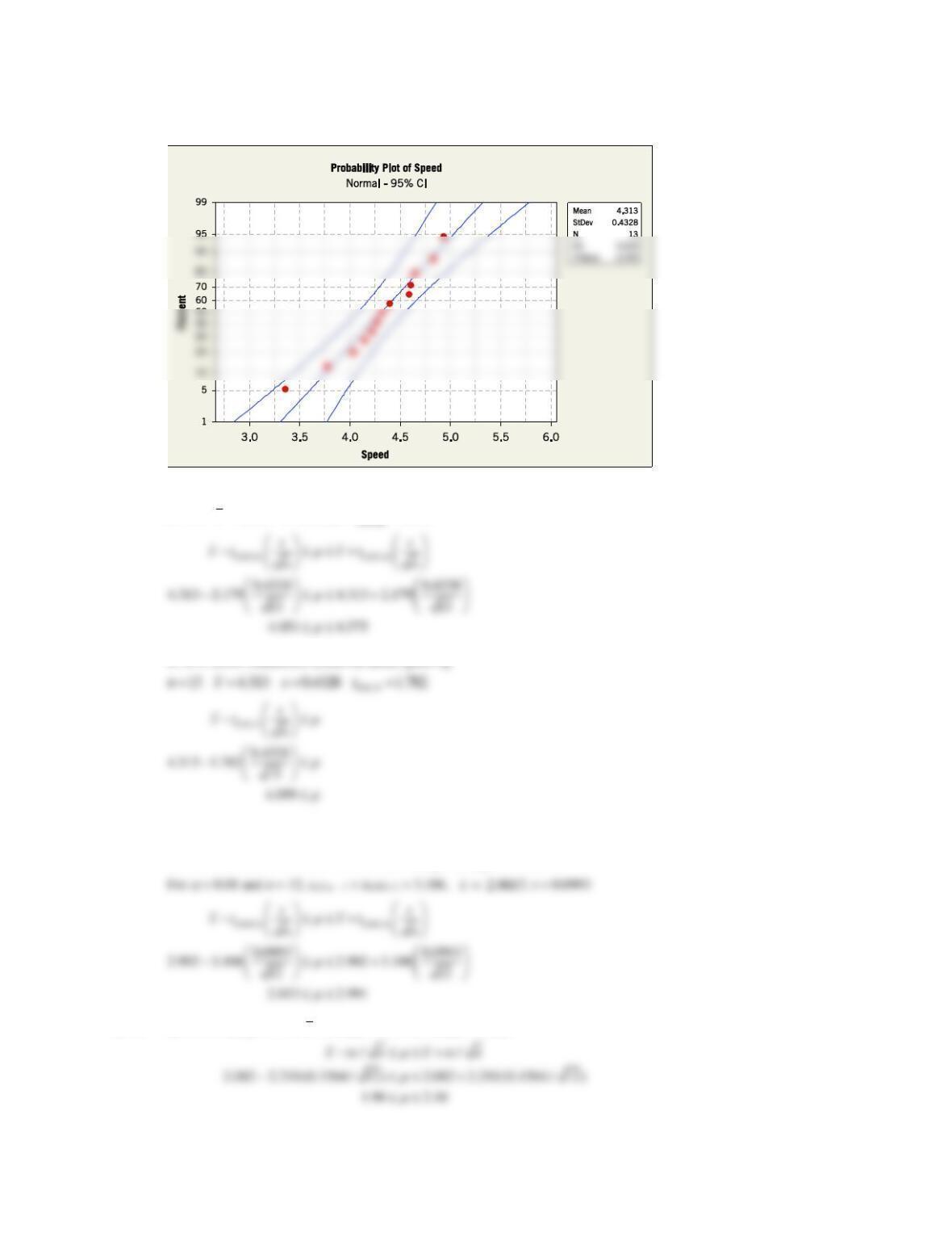
8.2.10 a) The data appear to be normally distributed based on examination of the normal probability plot below.
b) 95% confidence interval on mean speed-up
0.025,12
13 4.313 0.4328 2.179n x s t= = = =
c) 95% lower confidence bound on mean speed-up
8.2.11 a) The data appear to be normally distributed.
b) 99% two-sided confidence interval on mean percentage enrichment.
8.2.12 a) 95% CI for μ, n = 12,
2.082x=
, s = 0.1564, t0.025,11 = 2.201
Applied Statistics and Probability for Engineers, 7th edition 2017
8-8
b) The lower bound of 95% confidence interval is greater than the historical average of 1.95. Therefore, there is
Section 8.3
8.3.1 95% confidence interval for
given n = 51, s = 0.37
8.3.2
2
0.05,10 18.31
=
2
0.025,15 27.49
=
2
0.01,12 26.22
=
8.3.3 The data appear to be normally distributed based on examination of the normal probability plot below.
95% confidence interval for
Applied Statistics and Probability for Engineers, 7th edition 2017
8-9
8.3.4 95% confidence interval for
n = 17 s = 0.09
8.3.5 95% confidence interval for
n = 15 s = 0.00831
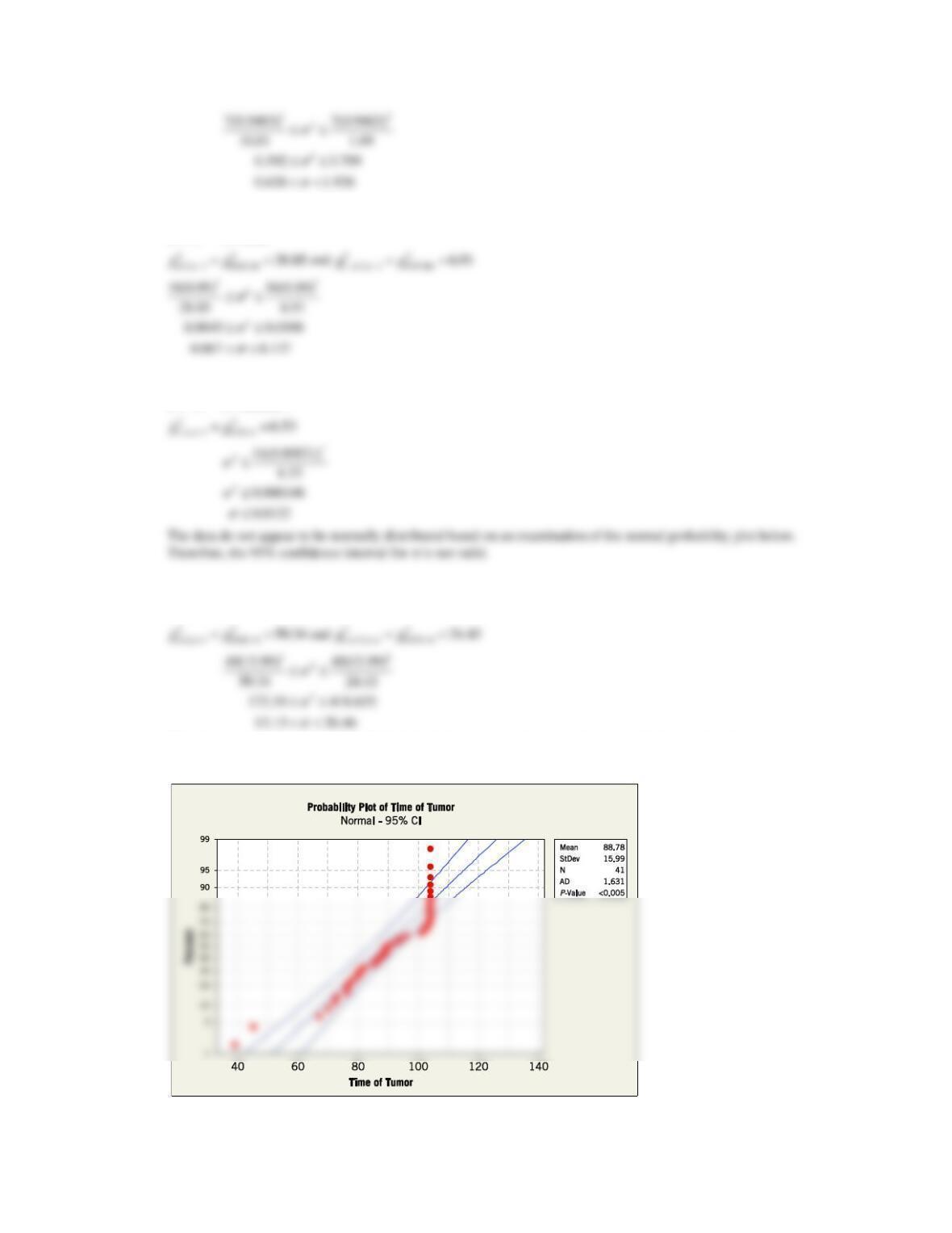
8.3.6 95% confidence interval for
n = 41 s = 15.99
The data do not appear to be normally distributed based on examination of the normal probability plot below.
Therefore, the 95% confidence interval for
is invalid.
Applied Statistics and Probability for Engineers, 7th edition 2017
8-10
8.3.7 95% two sided confidence interval for
, n = 39 s = 0.6295
Section 8.4
8.4.1 a) 95% confidence interval for the proportion of college graduates in Ohio that voted for George Bush.
/2
412
ˆ0.536 768 1.96
p n z
= = = =
8.4.2 a) 95% confidence interval on the proportion of such tears that will heal.
/2
ˆ0.676 37 1.96p n z
= = =
8.4.3 a) 95% confidence interval on the proportion of rats that are under-weight.
12
ˆ0.4
p==
n = 30
=z/2 1.96
Applied Statistics and Probability for Engineers, 7th edition 2017
8-11
8.4.4 The worst case would be for p = 0.5, thus with E = 0.05 and
= 0.01,
==zz
/2 0.005 2.58
we obtain a sample size of:
8.4.5 a)
466
ˆ0.932
500
p==
n = 500
=z/2 1.96
b) E = 0.01,
= 0.05,
==zz
/2 0.025 1.96
and
ˆ0.932p=
as the initial estimate of p,
c) E = 0.01,
= 0.05,
==zz
/2 0.025 1.96
8.4.6 a)
180
ˆ0.9
p==
n = 200
=z/2 1.96
==zz
/2 0.025 1.96
==zz
/2 0.025 1.96
Applied Statistics and Probability for Engineers, 7th edition 2017
8-12
Section 8.6
8.6.1 95% prediction interval on the life of the next tire given
60139.7x=
, s = 3645.94, n = 16
8.6.2 90% prediction interval the value of the natural frequency of the next beam of this type that will be tested. Givenx =
8.6.3 Given
317.2x=
, s = 15.7, n = 10 for
= 0.05 t/2,n − 1 = t0.005,9 = 3.250
8.6.4 90% prediction interval on the next specimen of concrete tested
8.6.5 90% prediction interval for enrichment data given
2.9x=
, s = 0.099, n = 12 for
= 0.10
Applied Statistics and Probability for Engineers, 7th edition 2017
8-13
The 90% confidence interval is
8.6.6 To obtain a one-sided prediction interval, use t,n − 1 instead of t
/2,n − 1
8.6.7 95% tolerance interval on the life of the tires that has a 95% CL
8.6.8 99% tolerance interval on the brightness of television tubes that has a 95% CL
8.6.9 90% tolerance interval on the comprehensive strength of concrete that has a 90% CL
8.6.10 99% tolerance interval on rod enrichment data that have a 95% CL
Applied Statistics and Probability for Engineers, 7th edition 2017
8-14
Supplemental Exercises
8.S7 Where
1 +
2 =
. Let
= 0.05
Interval for
1=
2 =
/2 = 0.025
8.S8 a) The data appear to follow a normal distribution based on the normal probability plot because the data fall along a
straight line.
8.S9 μ = 50,
2 = 5
a) For n = 16 find P(s2 ≥ 7.44) or P(s2 ≤ 2.56)
Applied Statistics and Probability for Engineers, 7th edition 2017
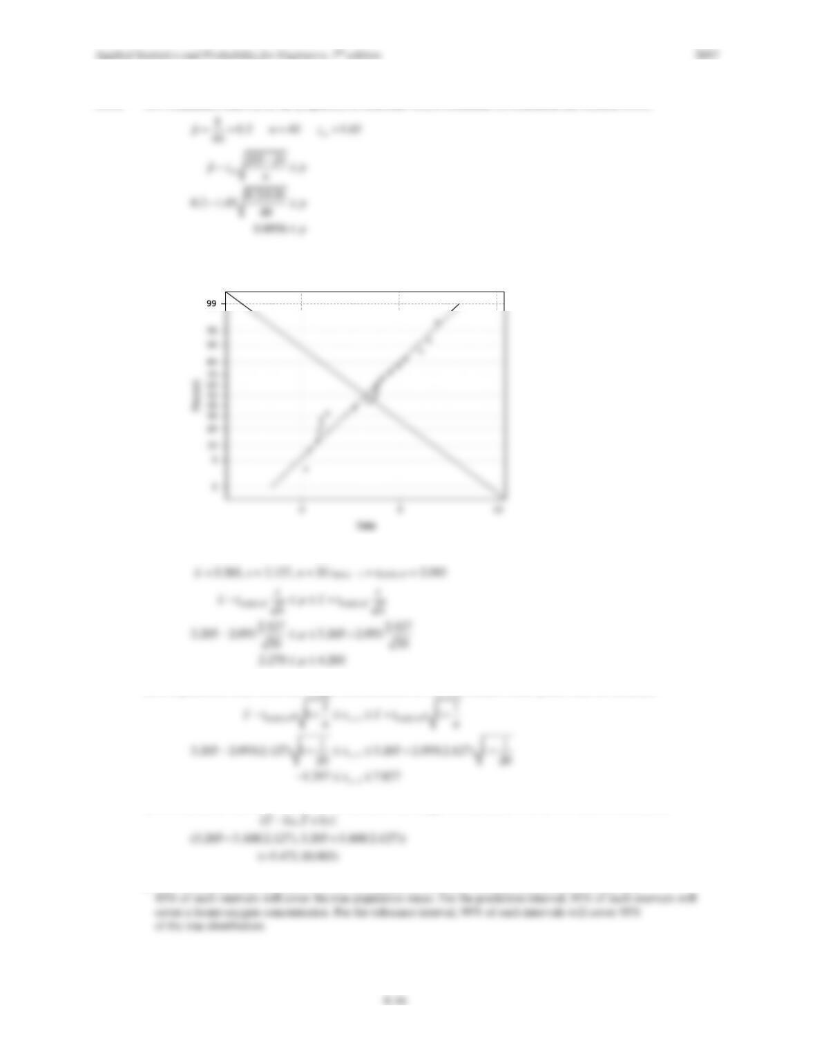
8.S10 a) Normal probability plot for the coefficient of restitution.
b) 99% CI on the true mean coefficient of restitution
c) 99% prediction interval on the coefficient of restitution for the next baseball that will be tested.
d) 99% tolerance interval on the coefficient of restitution with a 95% level of confidence
8.S11 95% confidence interval on the proportion of baseballs with a coefficient of restitution that exceeds 0.635.
8.S12 a) The normal probability shows that the data are mostly follow the straight line, however, there are some points that
deviate from the line near the middle.
b) 95% CI on the mean dissolved oxygen concentration
c) 95% prediction interval on the oxygen concentration for the next stream in the system that will be tested
d) 95% tolerance interval on the values of the dissolved oxygen concentration with a 99% level of confidence
e) The confidence interval in part (b) is for the population mean and we may interpret this to imply that
8.S13 99% confidence interval on the population proportion
= = = = =
ˆ
1600 8 0.005 2.58n x p z z
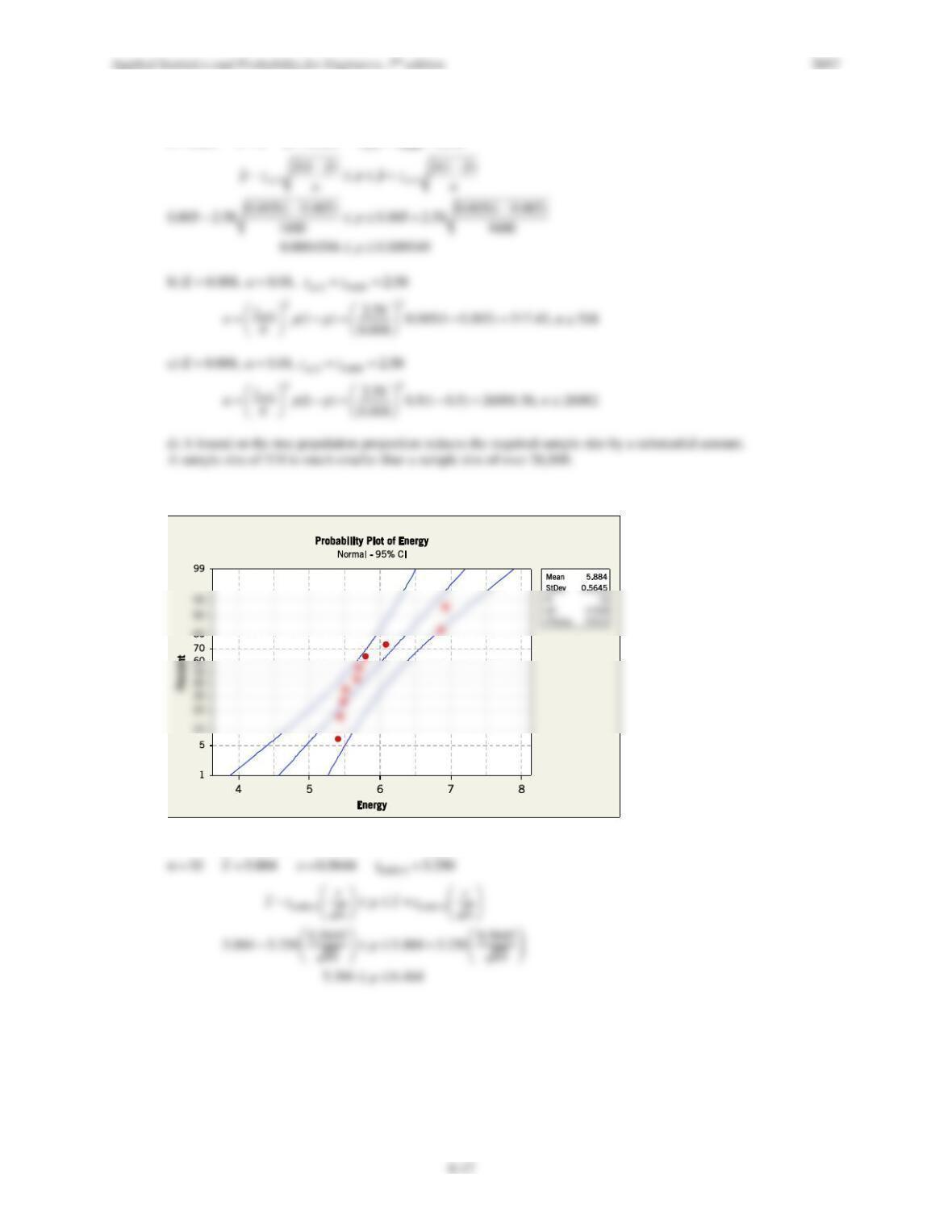
8.S14 a) The data appear to be normally distributed based on examination of the normal probability plot below.
b) 99% upper confidence interval on mean energy (BMR)