Applied Statistics and Probability for Engineers, 7th edition 2017
7-1
CHAPTER 7
Section 7.2
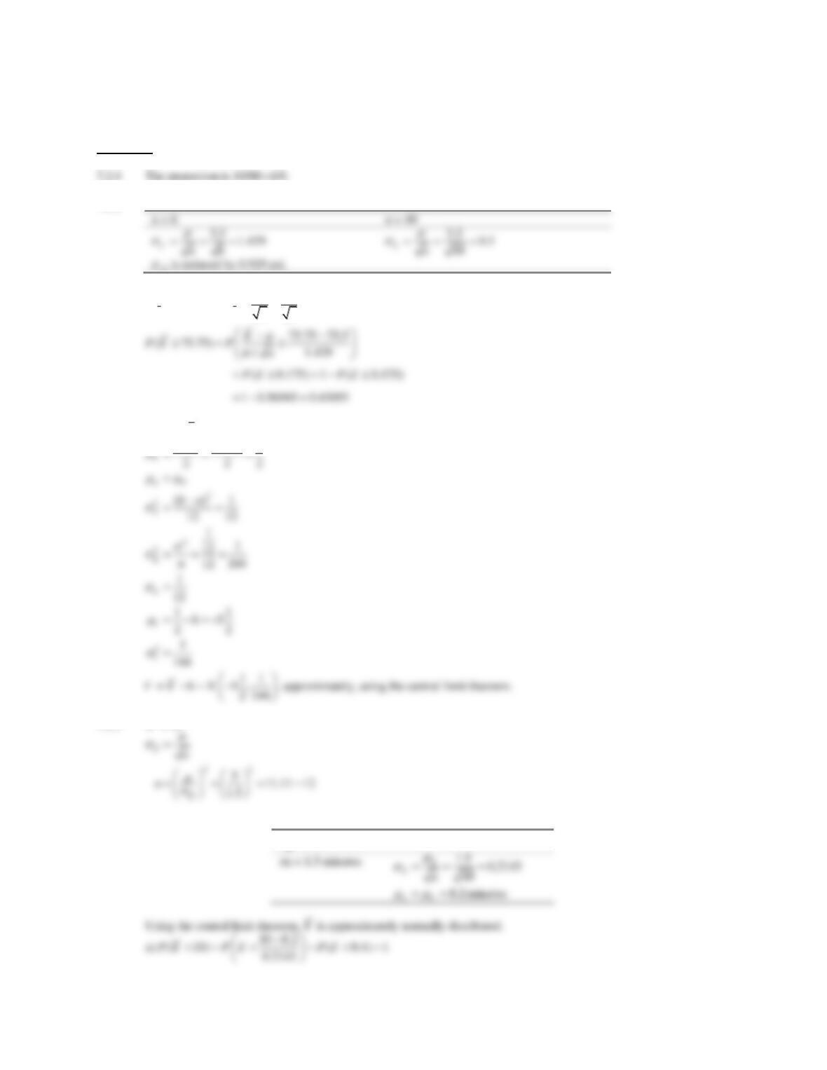
7.2.2
X
7.2.3
3.5
75.5psi 1.429
6
XX
n
= = = =
7.2.4 Let
6YX=−
++
(0 1) 1
ab
7.2.5
2 = 25
7.2.6
μX = 8.2 minutes
n = 49
Applied Statistics and Probability for Engineers, 7th edition 2017
7-2
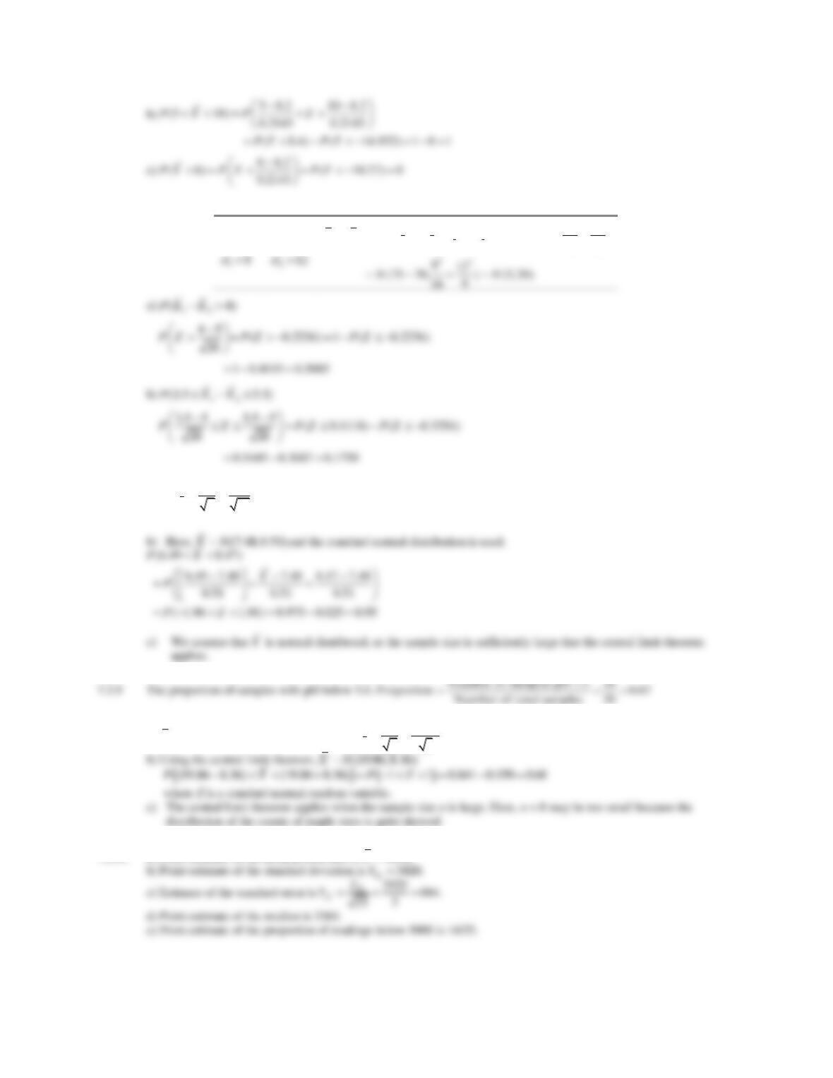
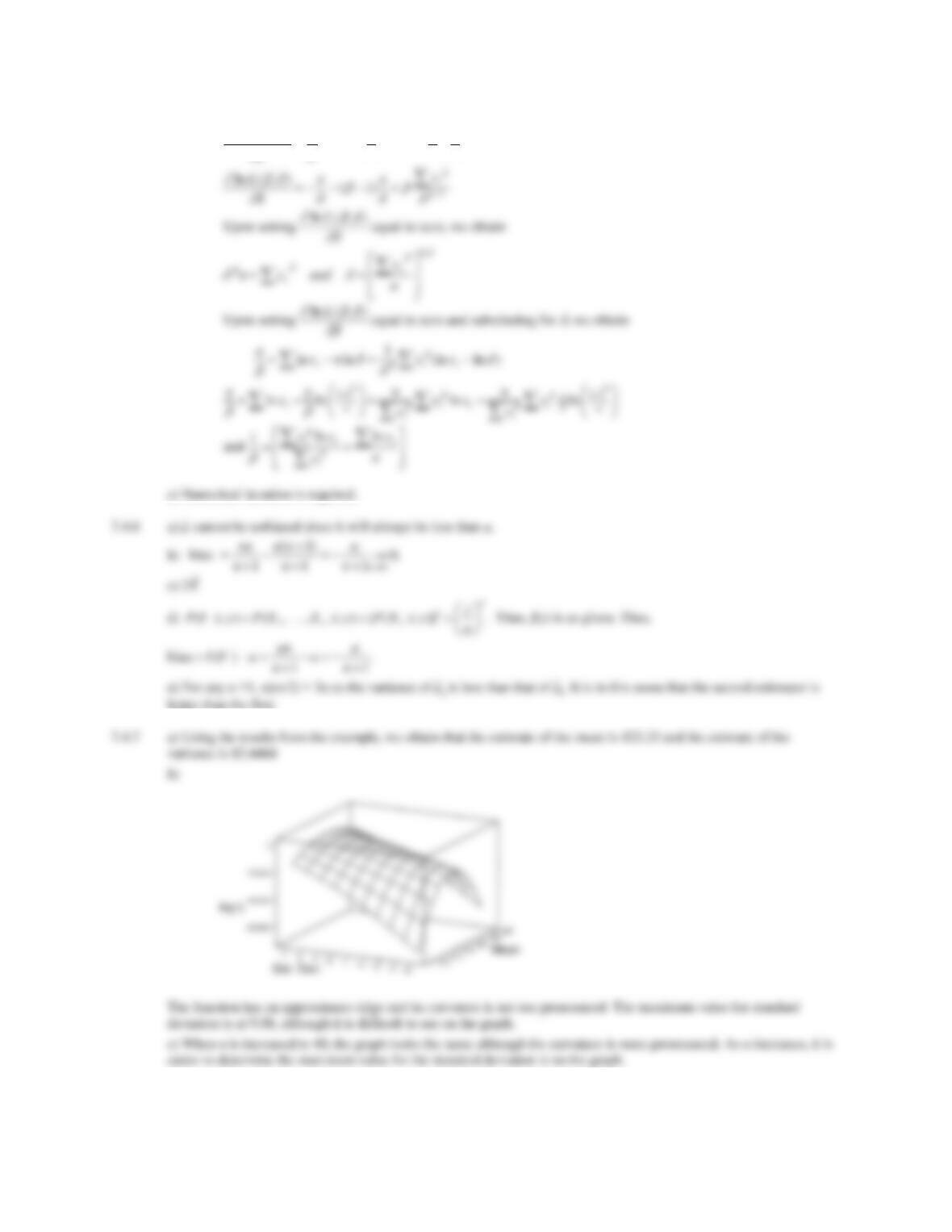
7.2.7
=
=
1
1
16
75
n
=
=
2
2
9
70
n
− − + − +
1
12
12
22
22 2
1 2 1 2 12
~ ( , ) ~ ( , )
XX
XX
X X N N nn
7.2.8 a)
= = =
1.60 0.51
10
X
X
SE n
7.2.10 a)
==19.86, 23.65
X
XS
, When n = 8,
= = =
23.65 8.36.
8
XX
s
SE n
7.2.11 a) Point estimate of the mean proton flux is
=4958.X
Applied Statistics and Probability for Engineers, 7th edition 2017
7-3
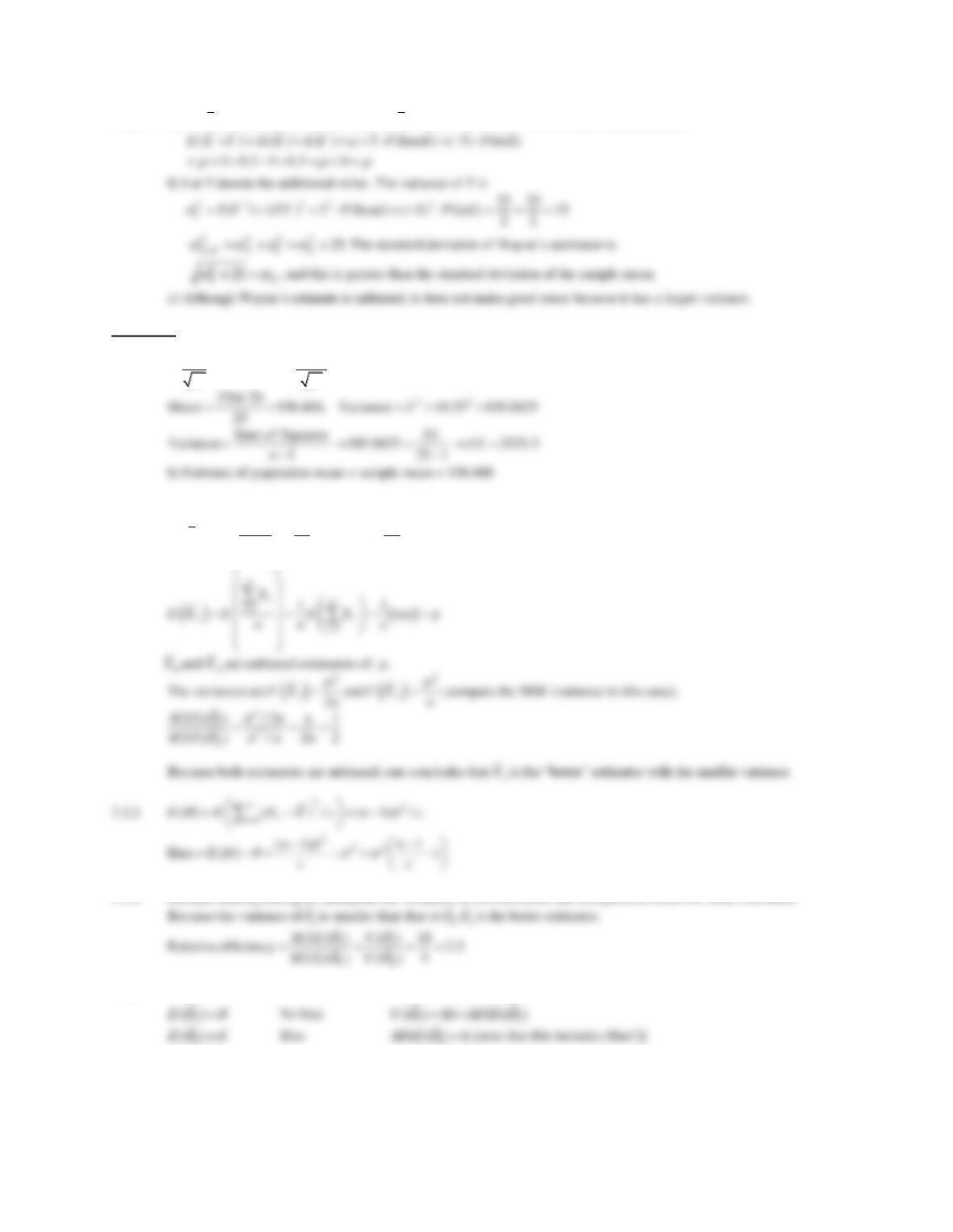
7.2.12 a) Let
X
denotes the mean miles and
=()E X
, we further let Y denotes the additional miles
Section 7.3
7.3.1 a)
= → = → =
10.25
SE Mean 2.05 25
SN
NN
7.3.2
( )
( )
=
=
= = = =
2
2
1
11
11
2
2 2 2
n
in
ii
i
X
E X E E X n
n n n
ˆ
ˆ
7.3.5
=
1
ˆ
()E
No bias
==
11
ˆˆ
( ) 12 ( )V MSE
3
ˆ
Applied Statistics and Probability for Engineers, 7th edition 2017
7-4
To compare the three estimators, calculate the relative efficiencies:
3
2
7.3.7
Variable N Mean Median TrMean StDev SE Mean
Oxide Thickness 24 423.33 424.00 423.36 9.08 1.85
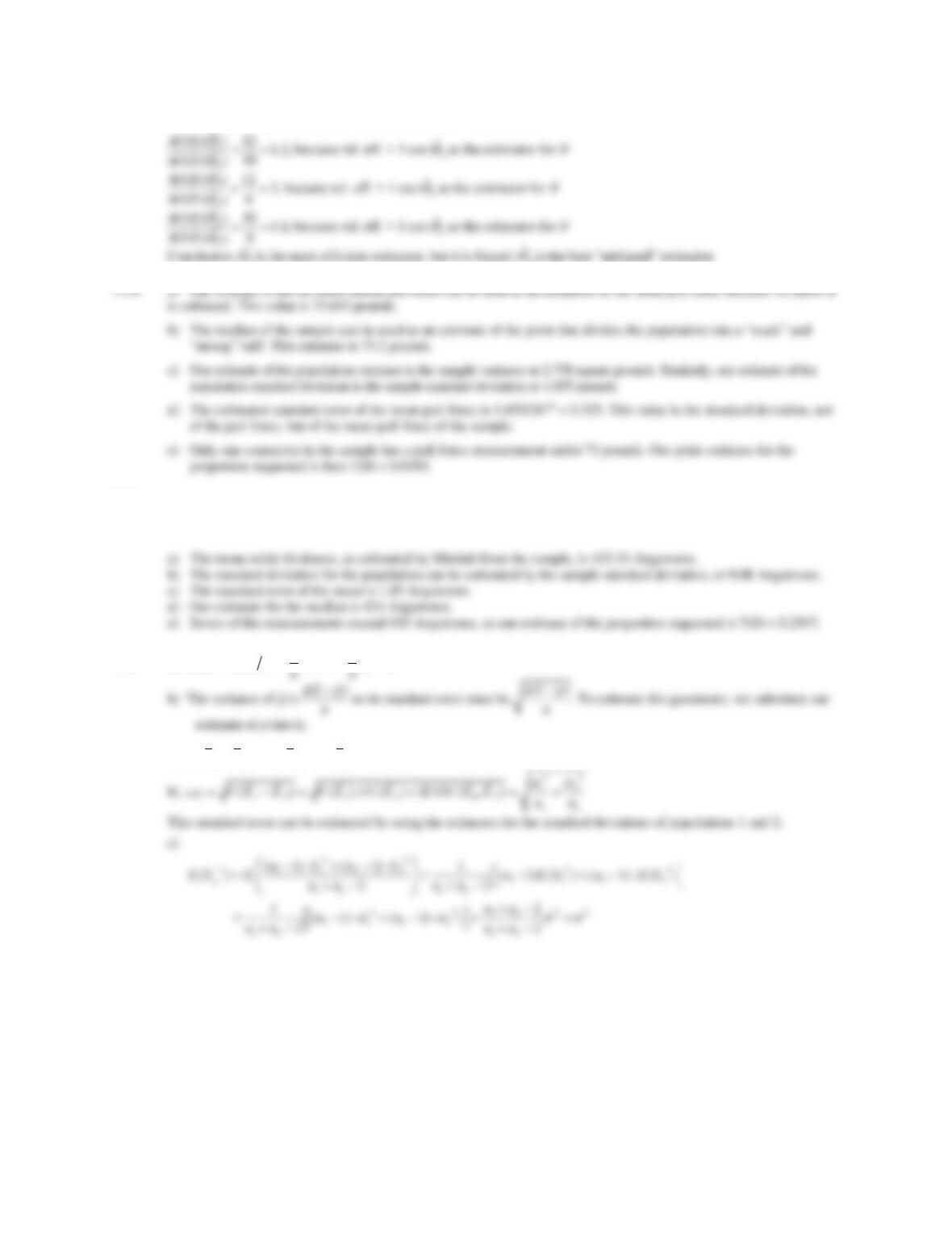
7.3.8 a)
= = = =
11
ˆ
( ) ( ) ( )E p E X n E X np p
7.3.9 a)
− = − = −
1 2 1 2 1 2
( ) ( ) ( )E X X E X E X
2
3
3
Applied Statistics and Probability for Engineers, 7th edition 2017
7-5
7.3.10 X ~ norm(μ = 10,
2 = 42), n = 16, nB = 200, the original sample (n = 16):
#
1
2
3
4
5
6
7
8
Value
4.26
6.59
12.36
7.47
10.84
1.17
17.02
14.10
7.3.11
a)
− = − = − = − = −
12 1 2 1 1 2 2 1 2 1 2
1 2 1 2 1 2
1 1 1 1
( ) ( ) ( )
XX
E E X E X n p n p p p E p p
n n n n n n
7.3.12 Suppose that two independent random samples (of size n1 and n2) from two normal distributions are available. Explain
how you would estimate the standard error of the difference in sample means
−
12
XX
with the bootstrap method.
Value
12.30
6.73
16.75
11.87
12.25
7.52
7.10
9.80
Applied Statistics and Probability for Engineers, 7th edition 2017
7-6
Section 7.4
7.4.1.
−
=− 1
( ) (1 )x
f x p p
7.4.3
=
−
= = =
1
01
() 2
n
i
i
a
E X X X
n
, therefore:
=
ˆ2aX
7.4.4 a)
−−
+ = = + =
1
12
11
(1 ) 1 ( ) 2
2
x
c x dx cx c c
7.4.5 a)
=
−−
−
−
==
==
1
11
11
(,)
ni
i
i
x
x
nn
ii
ii
xx
L e e
Applied Statistics and Probability for Engineers, 7th edition 2017
7-7
b)
( ) ( )( )
= + −
ln ( , ) ln ln
i i i
x x x
Ln
better than the first.
Applied Statistics and Probability for Engineers, 7th edition 2017
7-8
Supplemental Exercises
7.S13
7.S14
−
=
=
1
1
1
()
n
i
ni
Lx
Upon setting the last equation equal to zero and solving for the parameter of interest, we obtain the maximum
likelihood estimate
=−
1
ˆln( )
n
i
x
n
Applied Statistics and Probability for Engineers, 7th edition 2017
7.S15
+ + + +
= = =
23.1 15.6 17.4 28.7
ˆ21.86
10
x