110
CHAPTER 6 SPECIAL TOPICS: STATE REDUCTION AND HIDDEN MARKOV
CHAINS
6.1)
Matrix Reduction
3
12 4
1
1 0.23 0.34 0.26 0.17
S
ªº
3
24
(2) (2)
2 0.42 0.18 0.32 0.08
2 0.4553 0.2070 0.3377
ªºªº
ªº
ªº
¬¼
¬¼ ¿
Back Substitution produces the solution
111
4310
6.2)
01 0 0 0
1 0.08 0.42 0.18 0.32 1 0
2 0.31 0.17 0.23 0.29
3 0.24 0.36 0.34 0.06
M
ªº
«»
ªº
«»
«»
¬¼
«»
¬¼
A. Augmentation
(1) (1)
1 0.42 0.18 0.32 0.08 1
B. Matrix Reduction
1 0.42 0.18 0.32 0.08 1
ªº
ªº
C. Back Substitution produces the solution
»
º
«
ª
»
º
«
ª
7818.5
1
10
m
6.3)
112
A. Augmentation
»
º
«
ª
1514131211
1
ggggg
>@
)1(
1
)1(
15
)1(
14
)1(
13
)1(
12
)1()1()2(
)1()1(
12
15.025.01.03.02.0
1
ReductionMatrix B.
u
vTG
º
ª
»
«
gggg
35
34
33
)2()2(
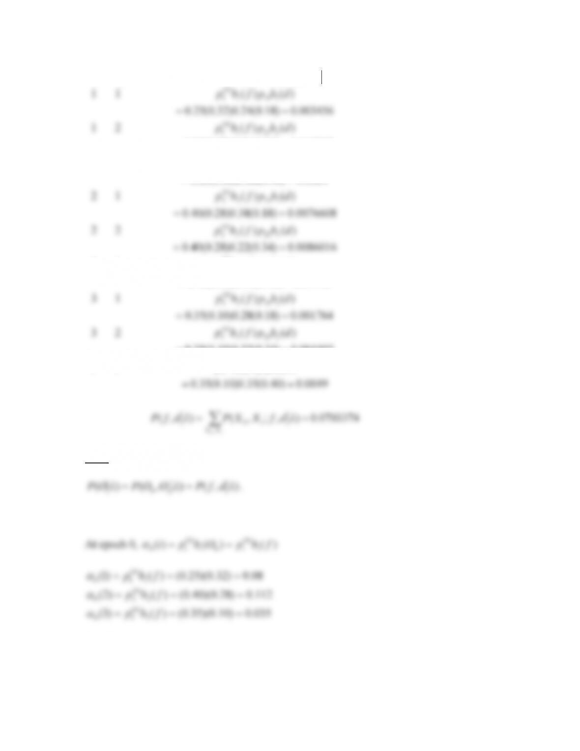
C. Back Substitution
Back substitution begins by computing the entry in row 3 of the vector of
probabilities of absorption in state 0.
4177.02886666.0402444.02886666.0
)3(
35
)3(
34
)3(
3530
gggf
Next the entry in row two is computed.
113
3511.010875.024125.02125.0)4177.0(2125.010875.0
)2(
25
)2(
24
)2(
2330
)2(
23
)2(
2520
gggfggf
Finally, the entry in row one is computed.
3714.015.025.01.03.0)4177.0(1.0)3511.0(3.015.0
)1(
15
)1(
14
)1(
13
)1(
1230
)1(
1320
)1(
12
)1(
1510
ggggfgfggf
The vector
0
f
of probabilities of absorption in absorbing state 0 is
»
»
»
¼
º
«
«
«
¬
ª
»
»
»
¼
º
«
«
«
¬
ª
4177.0
3511.0
3714.0
3
2
1
30
20
10
0
f
f
f
f
6.4)
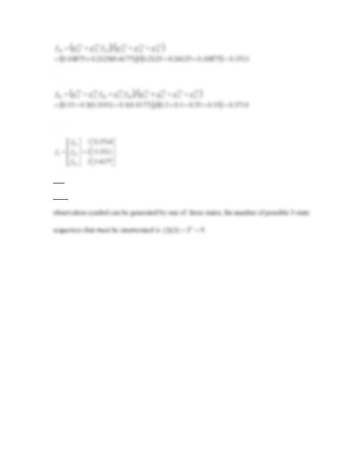
6.4a) Since the observation sequence consists of two observation symbols, and each
114
)()(11
),;,(y ProbabilitJoint
10 ,
10
1111
)0(
1
1010
¦
XX
dbpfbp
dfXXPXX
O
6.4b) The forward procedure will be executed to calculate
10
Step 1. Initialization.
)0(
035.0)10.0)(35.0()()3(
3
)0(
30
2
20
fbp
D
Step 2. Induction
115
At epoch 1,
)(])3()2()1([)(])([)(
302010
3
1
101
dbpppObpij
jjjj
ijij
DDDDD
¦
)(])3()2()1([)1( 13102101101
dbppp
DDDD
02922.0)40.0)](35.0)(035.0()40.0)(112.0()20.0)(08.0[(
Step 3. Termination
At epoch
1 M
,
3
6.4c) The Viterbi algorithm will be executed to recover the state sequence,
},{
10
XXX
, which has the highest probability of generating the observation sequence,
X
X
Step 1. Initialization.
At epoch 0,
)()()(
)0(
0
)0(
0
fbpObpi
iiii
G
.
08.0)32.0)(25.0()()1(
)0(
1
)0(
10
fbp
G
3
30
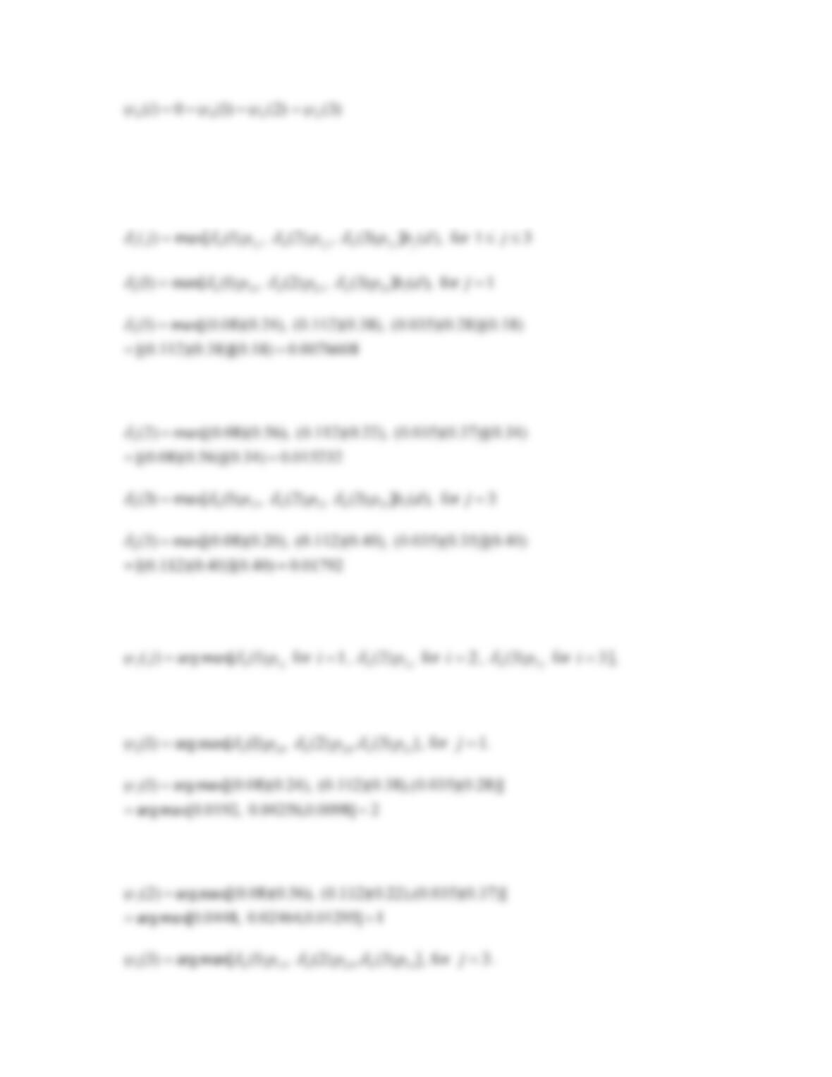
116
000
0
Step 2. Recursion
At epoch 1,
31for ),(])([max)(])([max)(
0
31
10
31
1
dd
dddd
jdbpiObpij
jij
i
jij
i
GGG
0076608.0)18.0)](38.0)(112.0[(
2for ),(])3( )2( ,)1([max)2(
23202201201
jdbppp
GGGG
)34.0)](37.0)(035.0( ),22.0)(112.0( ),56.0)(08.0[(max)2(
1
G
01792.0)40.0)](40.0)(112.0[(
31for ],)([argmax)(
0
31
1
dd
dd
jpij
ij
i
G
\
j
pj
101
)1([maxarg)(
G
\
for
1 i
,
j
p
20
)2(
G
for
2 i
,
j
p
30
)3(
G
for
3 i
],
for
31 dd j
2]0098.0,04256.0 ,0192.0max[arg
])3(,)2( ,)1([maxarg)2(
3202201201
ppp
GGG
\
, for
2 j
.
)]37.0)(035.0(),22.0)(112.0( ),56.0)(08.0[(maxarg)2(
1
\
117
2]01225.0,0448.0 ,016.0[maxarg
)]35.0)(035.0(),40.0)(112.0( ),20.0)(08.0[(maxarg)3(
1
\
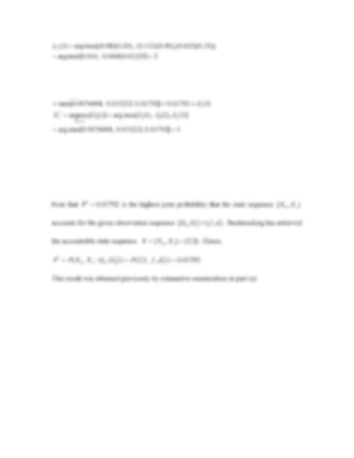
Step 3. Termination
3]0.01792 ,015232.0 ,0076608.0[maxarg
)3(01792.0]0.01792 ,015232.0 ,0076608.0[max
)]3( ),2( ),1([max)]([max
1111
1
1
1111
31
dd
G
GGGG
iP
i
Step 4. Backtracking to recover the state sequence
0for ,2)3()()(
00),11(for ),(
11110100
11
nXXX
nXX nnn
\\\
\
* P