5.8)
5.8a) The recurrent MDP model of virus removal with LP variables added in the right most
column is summarized below.
,,,
1
2
F 1=Do nothing 0.45 0.40 0.15 $0
M 2 Virus removal by A 0.64 0.28 0.08 280
kkk kk
iF iB iM i i
F
M
ikpppqy
y
y
3
M
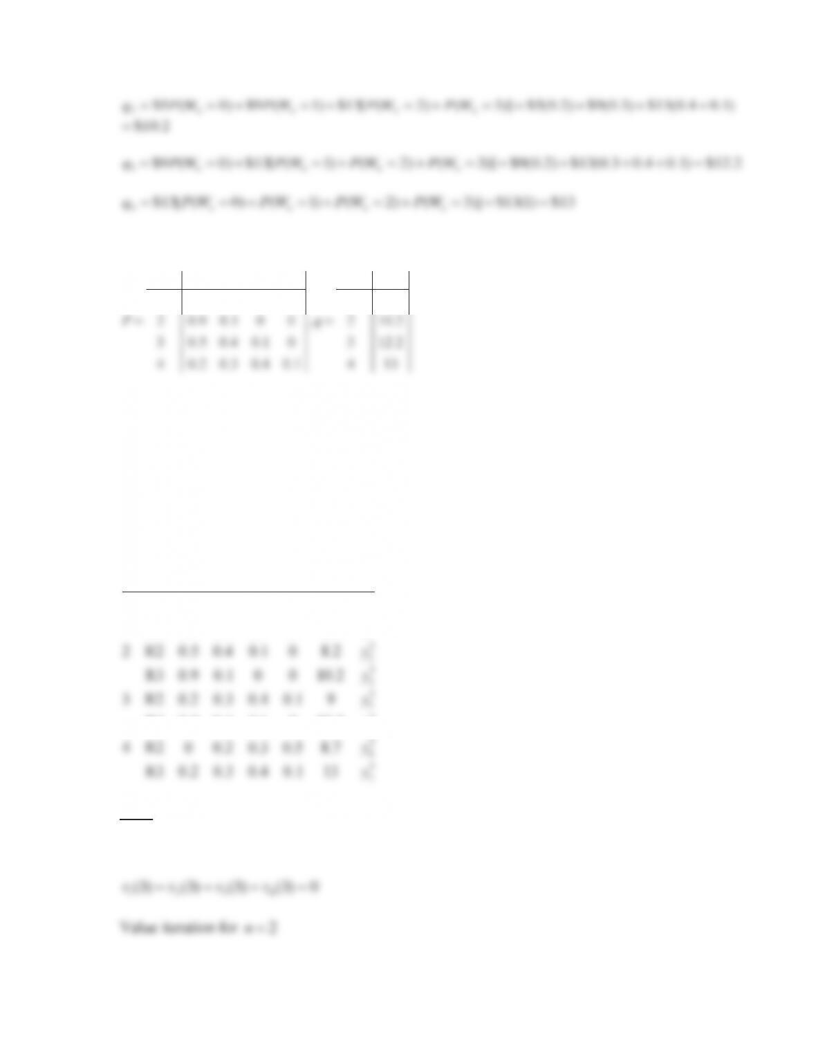
5.8b) To begin value iteration, assume zero expected total costs are incurred in every
state at the end of day 3.
123
(3) (3) (3) 0vvv
Value iteration for
2n
State
1
i
q
2
i
q
3
i
q
Expected Total Cost
Decision
i
1 k
2 k
3k
123
(2) min[ , , ]
iiii
k
vqqq
, for
1, 2, 3i
k
1=F
0
–
–
(2) 0v
1
–
160
110
3
–
280
200
3
95
Value iteration for
0n
i
k
12 3
(74) (155.4) (275.8)
kk k k
ii i i
qp p p
(0)
i
v
(0)
i
dk
1
1
0+0.45(74)+0.40(155.4)+0.15(275.8)=136.83←
1(0) 136.83v
1(0) 1d
2
2
160+0.92(74)+0.08(155.4)+0(275.8)=240.51
2
3
110+0.62(74)+0.34(155.4)+0.04(275.8)=219.75←
2
(0) 219.75v
2
(0) 3d
3
2
280+0.64(74)+0.28(155.4)+0.08(275.8)= 392.94
3
3
200+0.45(74)+0.38(155.4)+0.17(275.8) =339.24←
3
(0) 339.24v
3
(0) 3d
An optimal policy over the next three days is summarized below.
1
2
0123
( ) 136.83 74 0 0
() 3 3 3
n
vn
dn
5.8c) After omitting the last constraint which is redundant, the linear programming
formulation for the recurrent MDP model of virus removal appears below.
FBB MM
subject to
123 23
1) 0.55 ( 0.92 0.62 ) ( 0.64 0.45 ) 0
FBB MM
yy y y
96
Objective function value, g 63.47
k
i
iky
Row Dual Variable
Constraint 1 202.39
F
v
The optimal policy is given by the vector
[1 3 3]
T
d
. Under this policy, a virus is
always removed by consultant B. The minimum expected average cost per month is
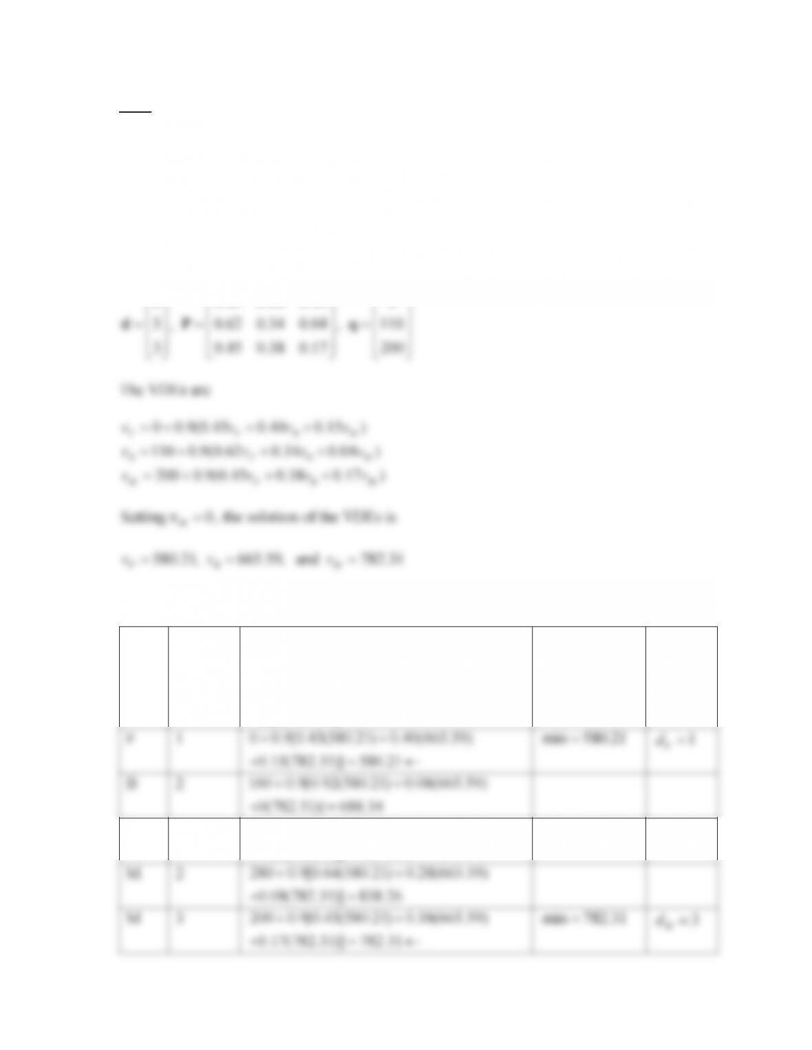
5.8d) To begin policy iteration, arbitrarily choose the initial policy
[1 3 3]
T
d
. The
initial decision vector
d
, along with the associated transition probability matrix
P
and
the cost vector
q
, are shown below.
1 0.45 0.40 0.15 0
ªº ª º ª º
¬¼ ¬ ¼ ¬ ¼
The VDEs are
0 0.45 0.40 0.15
FFBM
gv v v v
Setting v 0
M
, the solution of the VDEs is
FB M
First policy improvement for virus removal model
State Decision Test Quantity
State
i
Decision
Alterna-
tive
k
Test Quantity
( 202.39) ( 119.62) (0)
kk k k
iiFFiBBiMM
kk k k
iiF iB iM
qpvpvpv
qp p p
Minimum
Value of
Test
Quantity
Decision
kdi
F
1
0 0.45( 202.39) 0.40( 119.62)
138.92
m
min 138.92
1
F
d
98
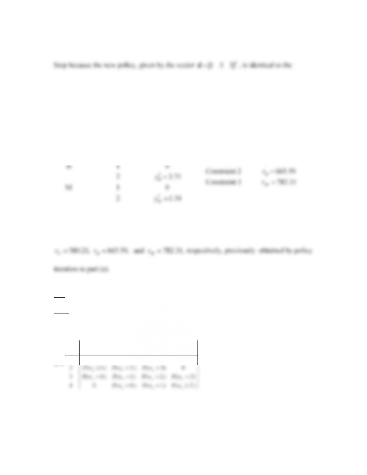
5.8e) Begin policy iteration with
0.9
D
by choosing an initial policy given by the
vector.
[1 3 3]T
d
.
The initial decision vector
d
, along with the associated transition probability matrix
P
and the cost vector
q
, are shown below.
1 0.45 0.40 0.15 0
ªº ª º ª º
First policy improvement for virus removal model
State Decision Test Quantity
State
i
Decision
Alterna-
tive
k
Test Quantity
()
0.9[ (580.21) (665.59)
(782.31)]
kk kk
iiFFiBBiMM
kk k
iiF iB
k
iM
qpvpvpv
qp p
p
D
Minimum
Value of
Test
Quantity
Decision
kd
i
F
1
0 0.9[0.45(580.21) 0.40(665.59)
0.15(782.31)] 580.21
m
min 580.21
1
F
d
B
2
160 0.9[0.92(580.21) 0.08(665.59)
0(782.31)] 688.34
B
3
110 0.9[0.62(580.21) 0.34(665.59)
0.04(782.31)] 665.59
m
min 665.59
3
B
d
2
0.08(782.31)] 838.26
M
3
200 0.9[0.45(580.21) 0.38(665.59)
0.17(782.31)] 782.31
m
min 782.31
3
M
d
99
previous policy. Therefore, this policy is optimal.
The linear programming solution for the discounted MDP machine maintenance
model with
0.9
D
appears below.
1
Objective function value, z 675.36
F 1 4.95
k
i
F
iky
y
Row Dual Variable
Constraint 1 580.21
F
v
Note that the dual variables associated with LP constraints 1, 2, and 3, respectively, are
identical to the expected total discounted rewards,
5.9)
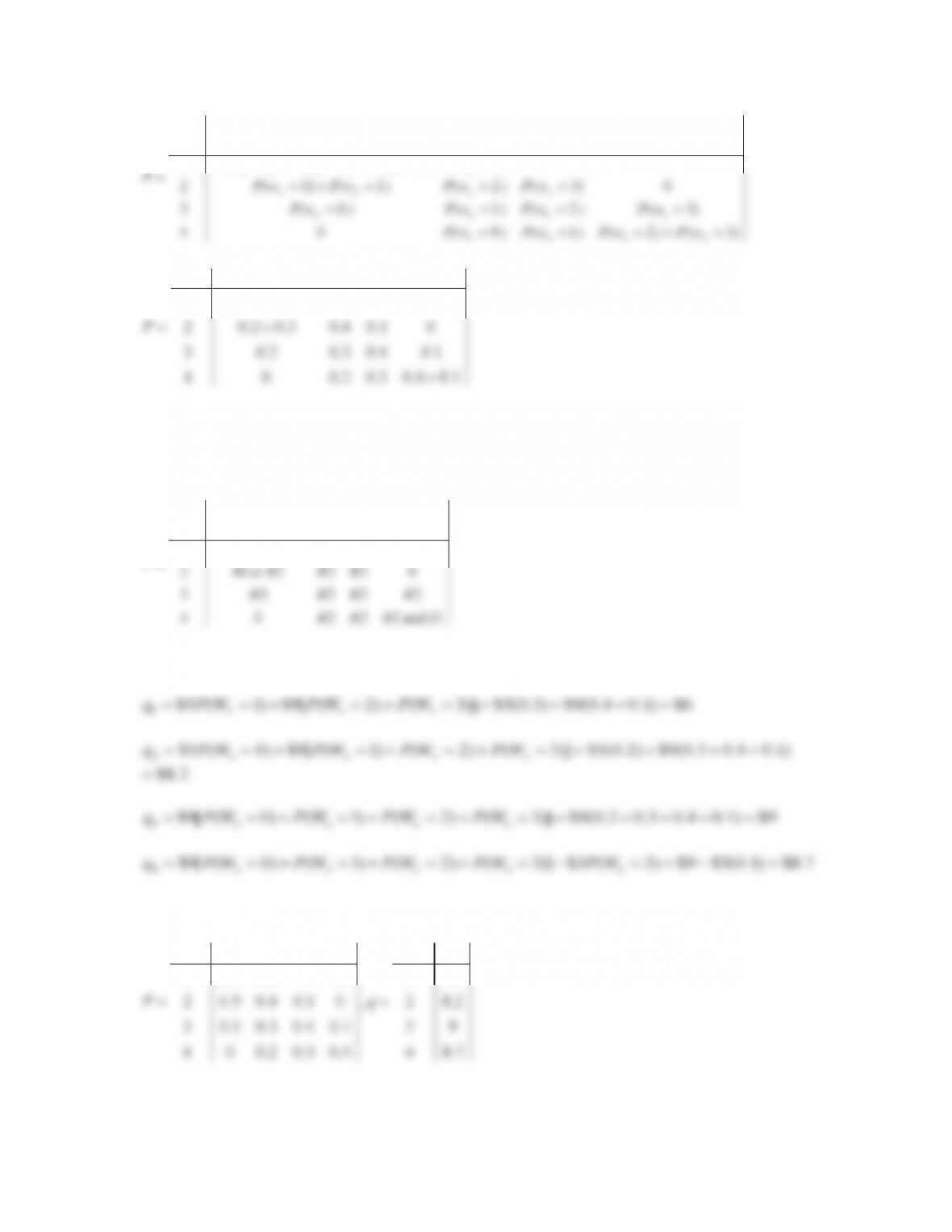
5.9a) Suppose that the decision is made to release up to 2 units of water at the beginning
of every week.
)P(w)P(w)P(w
wP)P(w)P(w)P(w
)P(w)P(w
nnn
nnnn
nn
21004
)3(2103
00321
4321State
t
d
100
)3(21004
)3(2103
0032)1()0(1
4321State
nnnn
nnnn
nnnn
wP)P(w)P(w)P(w
wP)P(w)P(w)P(w
)P(w)P(wwPwP
1.04.03.02.004
1.04.03.02.03
01.04.03.02.02
001.04.03.02.01
4321State
P
In the matrix below,
kR
denotes the release of
k
units of water, and
kS
denotes the
spilling away of
k
units of surplus water.
1 and 22204
22223
0222or 12
0022or 1or 01
4321State
SRRR
RRRR
RRRR
RRRR
P
The expected rewards in every state are calculated below.
4 nnnnn WPWPWPWPWPq
The MCR for the volume of water in the dam under the decision to release up to 2 units is
State 1 2 3 4
1 0.9 0.1 0 0 1 6
State
101
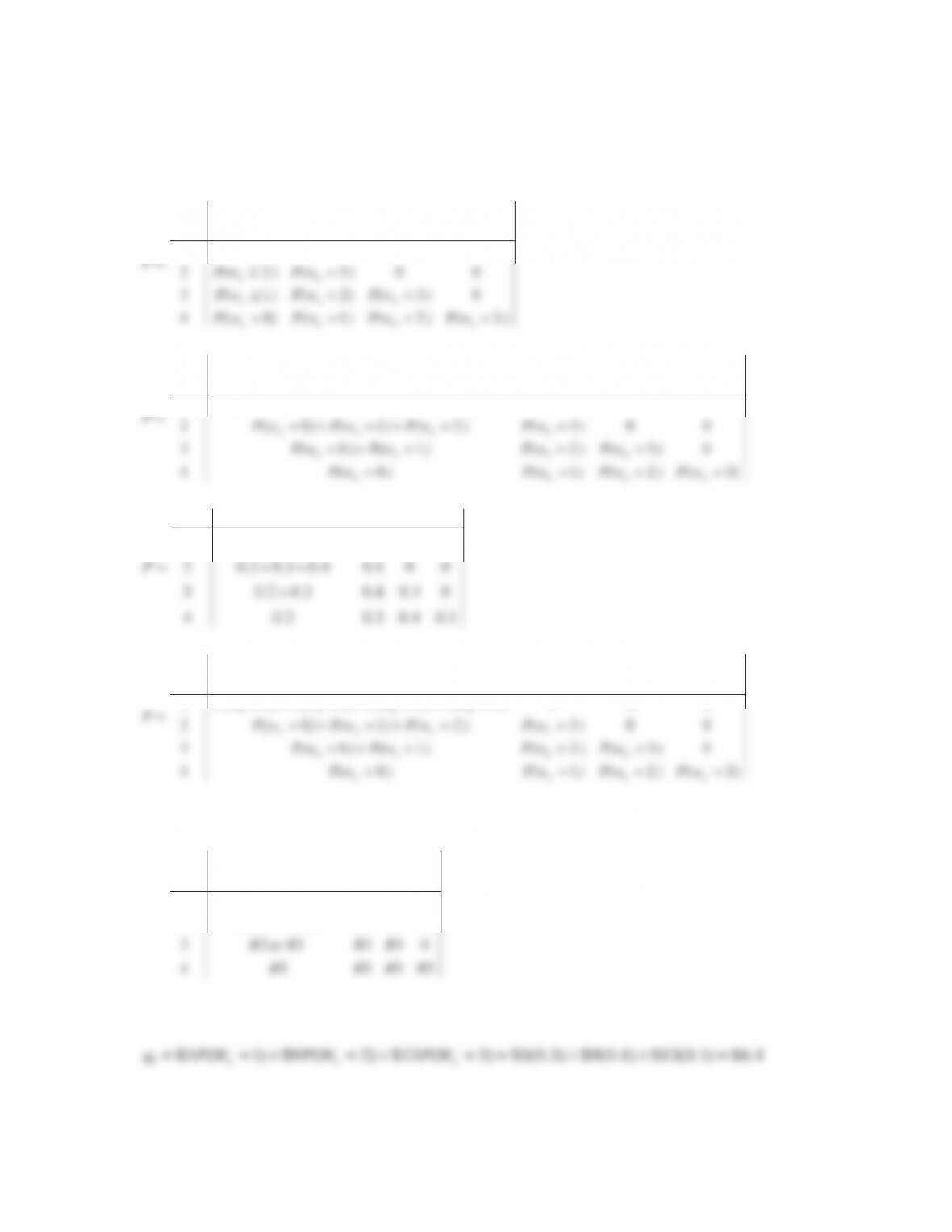
Now suppose that the decision is made to release up to 3 units of water at the
beginning of every week.
)P(w)P(w)P(wwP
)P(wP(w)P(w
)P(w
nnnn
nnn
n
321)0(4
03)213
00031
4321State
d
d
)3(2104
032103
00032)1()0(1
4321State
nnnn
nnnn
nnnn
wP)P(w)P(w)P(w
)P(w)P(w)P(w)P(w
)P(w)P(wwPwP
0001.04.03.02.01
4321State
)3(2104
032103
nnnn
nnnn
wP)P(w)P(w)P(w
)P(w)P(w)P(w)P(w
In the matrix below,
kR
denotes the release of
k
units of water.
3333 4
0333or 23
0033or 2or 12
0003or 2or 1or 01
4321State
RRRR
RRRR
RRRR
RRRR
P
The expected rewards in every state are calculated below.
1
nnn
102
)1.04.0(13$)3.0(9$)2.0(5$)]3()2([13$)1(9$)0(5$
2
nnnn WPWPWPWPq
4
nnnn
The MCR for the volume of water in the dam under the decision to release up to 3 units is
State 1 2 3 4
1 1 0 0 0 1 6.4
State
The unichain MDP model with LP variables added in the right most column is summarized
below.
Data for unichain MDP model of a dam
Reward
yProbabilit
Transition
DecisionState
1234
2
1
3
1
3
3
1R20.90.1 0 0 6
R3 1 0 0 0 6.4
R3 0.5 0.4 0.1 0 12.2
kk kk k k
ii ii i i
ik p p p p q y
y
y
y
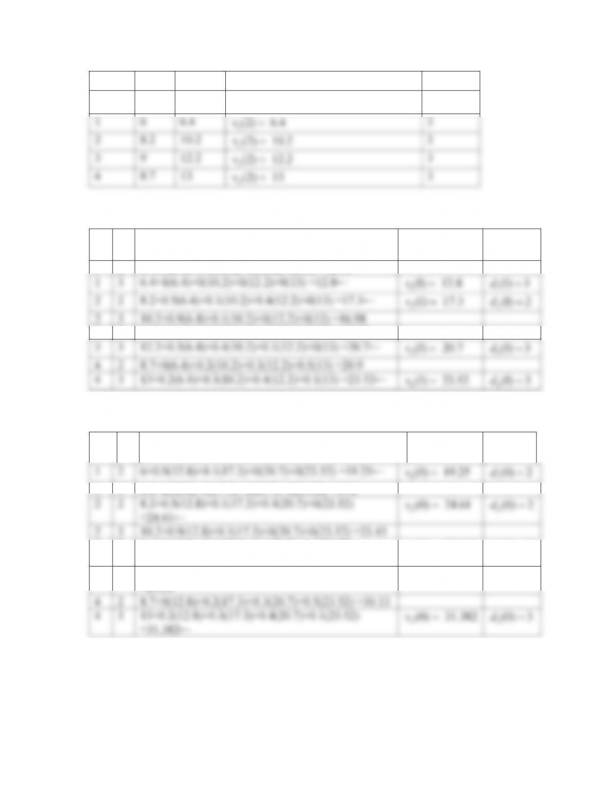
5.9b) To begin value iteration, assume zero expected total rewards are received in every
state at the end of week 3.
(3) (3) (3) (3) 0vvvv
State
2
i
q
3
i
q
Expected Total Reward
Decision
i
2k
3k
23
(2) max[ , ]
iii
k
vqq
, for
1, 2, 3, 4i
k
1
6
6.4
1(2) 6.4v
3
2
8.2
10.2
2(2) 10.2v
3
3
9
12.2
3
(2) 12.2v
3
4
8.7
13
4
(2) 13v
3
Value iteration for
1n
i
k
1234
(6.4) (10.2) (12.2) (13)
kk k k k
ii i i i
qp p p p
(1)
i
v
(1)
i
dk
1
2
6+0.9(6.4)+0.1(10.2)+0(12.2)+0(13) =12.78
1
3
6.4+1(6.4)+0(10.2)+0(12.2)+0(13) =12.8←
1(1) 12.8v
1
(1) 3d
2
2
8.2+0.5(6.4)+0.1(10.2)+0.4(12.2)+0(13) =17.3←
2
(1) 17.3v
2
(1) 2d
2
3
10.2+0.9(6.4)+0.1(10.2)+0(12.2)+0(13) =16.98
3
2
9+0.2(6.4)+0.3(10.2)+0.4(12.2)+0.1(13) =19.52
3
3
12.2+0.5(6.4)+0.4(10.2)+0.1(12.2)+0(13) =20.7←
3
(1) 20.7v
3(1) 3d
4
2
8.7+0(6.4)+0.2(10.2)+0.3(12.2)+0.5(13) =20.9
4
3
13+0.2(6.4)+0.3(10.2)+0.4(12.2)+0.1(13) =23.52←
4
(1) 23.52v
4(1) 3d
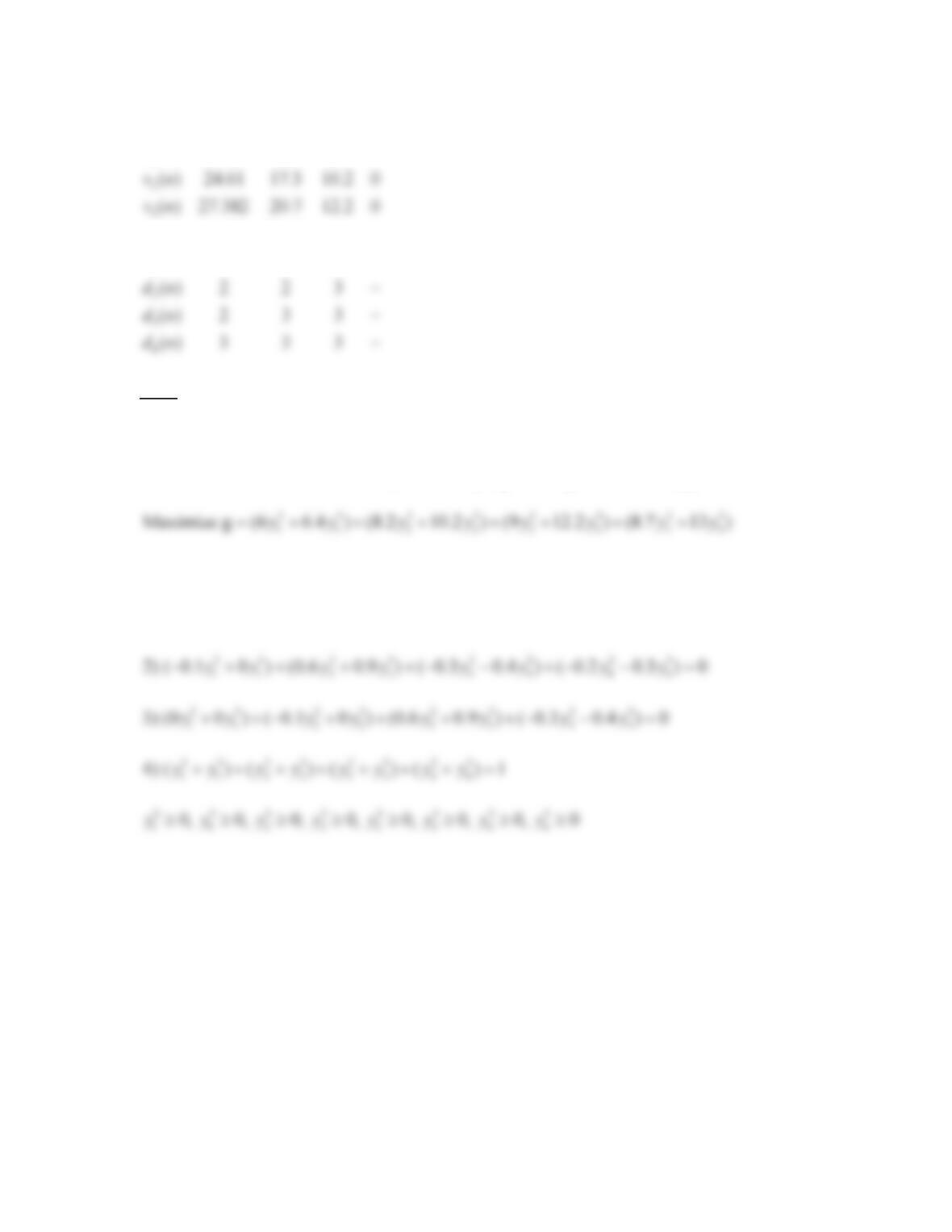
Value iteration for
0n
i
k
123 4
(12.8) (17.3) (20.7) (23.52)
kk k k k
ii i i i
qp p p p
(0)
i
v
(0)
i
dk
1
2
6+0.9(12.8)+0.1(17.3)+0(20.7)+0(23.52) =19.25←
1
(0) 19.25v
1
(0) 2d
1
3
6.4+1(12.8)+0(17.3)+0(20.7)+0(23.52) =19.2
2
2
8.2+0.5(12.8)+0.1(17.3)+0.4(20.7)+0(23.52)
=24.61←
2(0) 24.61v
2(0) 2d
2
3
10.2+0.9(12.8)+0.1(17.3)+0(20.7)+0(23.52) =23.45
3
2
9+0.2(12.8)+0.3(17.3)+0.4(20.7)+0.1(23.52)
=27.382←
3
(0) 27.382v
3
(0) 2d
3
3
12.2+0.5(12.8)+0.4(17.3)+0.1(20.7)+0(23.52)
=27.59
4
2
8.7+0(12.8)+0.2(17.3)+0.3(20.7)+0.5(23.52) =30.13
4
3
13+0.2(12.8)+0.3(17.3)+0.4(20.7)+0.1(23.52)
(0) 31.382v
(0) 3d
=31.382←
104
1
4
1
0123
( ) 19.25 12.8 6.4 0
( ) 31.382 23.52 13 0
() 2 3 3
n
vn
vn
dn
5.9c) The unichain MDP model of a dam will be formulated as a linear program to find a
release policy which maximizes the expected average reward or gain. After omitting the
last constraint which is redundant, the linear programming formulation appears below.
11 2233 44
subject to
23 23 2323
11 22 3344
1) (0.1 0 ) ( 0.5 0.9 ) ( .2 0.5 ) (0 0.2 ) 0yy yy yyyy
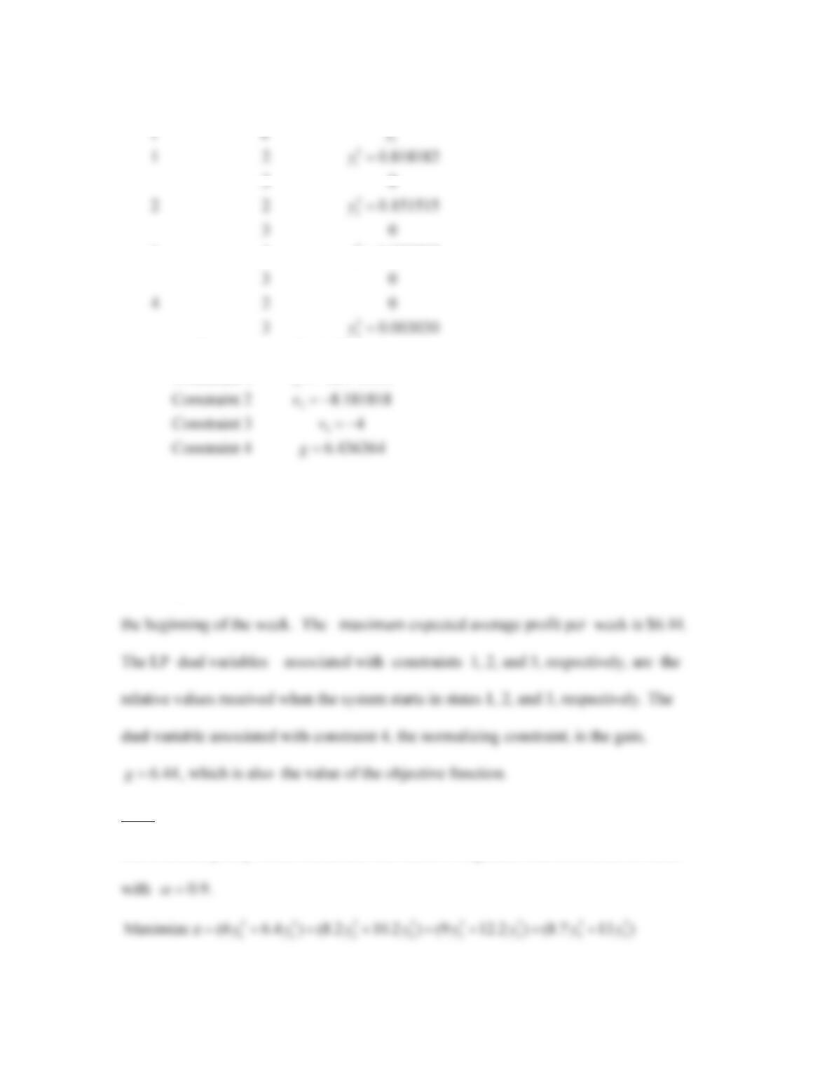
The solution of the unichain LP model is summarized below.
105
2
3
Objective function value, g 6.436364
3 2 0.272727
k
ik y
y
Row Dual Variable
Constraint 1 12.545455
v
The optimal policy is given by the vector
[2223]
T
d
. Under this policy, up to 2
units of water are released when 1, 2, or 3 units of water are stored in the dam at the
beginning of the week, and up to 3 units are released when 4 units of water are stored at
5.9d) The MDP model of a dam will be formulated as the following linear program to
find a release policy which maximizes the vector of expected total discounted rewards
11 2233 44
106
subject to
23 23 2323
11 22 3344
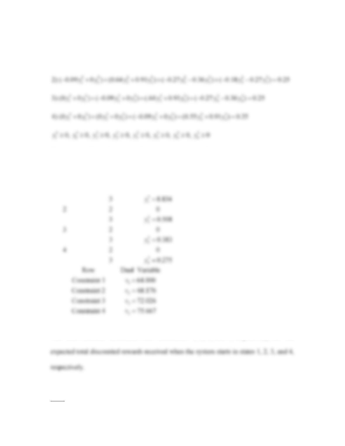
1) (0.19 0.10 ) ( 0.45 0.81 ) ( .18 0.45 ) (0 0.18 ) 0.25yy yy yyyy
The solution of the discounted LP model is summarized below.
Objective function value, z 69.967
12 0
k
i
iky
Row Dual Variable
Constraint 1 64.000
v
The dual variables associated with constraints 1, 2, 3, and 4, respectively, are the
5.10)
107
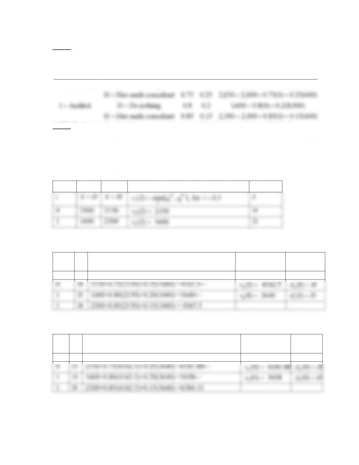
5.10a)
CostyProbabilit TransitionDecisionState
)600(15.0)0(85.0000,2300,215.085.0consultantaudit HireH
)000,8(2.0)0(8.0600,12.08.0nothing DoDAudited1
)000,8(3.0)0(7.0
400,2$3.07.0nothing DoDauditedNot 0
10
k
i
k
i
k
iqppki
5.10b) To begin value iteration, assume zero expected total costs are incurred in both
states at the end of year 3.
01
(3) (3) 0vv
Value iteration for
2n
State
D
i
q
H
i
q
Expected Total Cost
Decision
i
kD
kH
(2) min[ , ]
DH
iii
k
vqq
, for
0,1i
k
0
2400
2150
0(2) 2150v
H
1
1600
2300
1
(2) 1600v
D
Value iteration for
1n
i
k
01
(2150) (1600)
kk k
ii i
qp p
(1)
i
v
(1)
i
dk
0
D
2400+0.70(2150)+0.30(1600) =4385
0
H
2150+0.75(2150)+0.25(1600) =4162.5←
0(1) 4162.5v
0
(1)dH
1
D
1600+0.80(2150)+0.20(1600) =3640←
1(1) 3640v
1(1)dD
1
H
2300+0.85(2150)+0.15(1600) = 4367.5
Value iteration for
0n
i
k
01
(4162.5) (3640)
kk k
ii i
qp p
(0)
i
v
(0)
i
dk
0
D
2400+0.70(4162.5)+0.30(3640) =6405.75
0
H
2150+0.75(4162.5)+0.25(3640) =6181.88←
0
(0) 6181.88v
0
(0)dH
1
D
1600+0.80(4162.5)+0.20(3640) =5658←
1
(0) 5658v
1
(0)dD
1
H
2300+0.85(4162.5)+0.15(3640) =6384.13
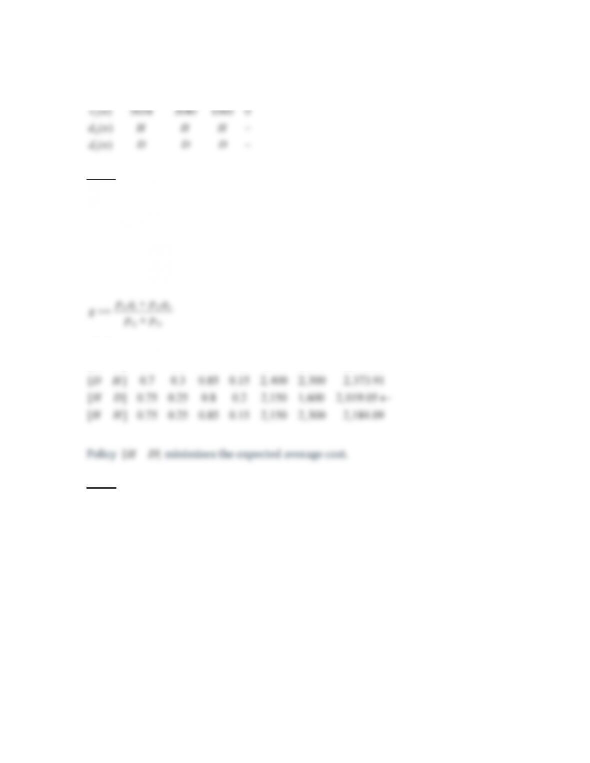
An optimal policy over the next three days is summarized below.
108
0
0123
( ) 6181.88 4162.5 2150 0
n
vn
5.10c) To use exhaustive enumeration, choose the policy which minimizes the expected
average cost, or negative gain, of the MCR which corresponds to each of the 4 alternative
policies. The expected average costs of the 4 alternative recurrent MCRs are calculated
using equation (4.65) below.
12 21
pq pq
00 01 10 11 0 1
Policy
[ ] 0.7 0.3 0.8 0.2 2,400 1,600 2,181.82
pppp q q g
DD
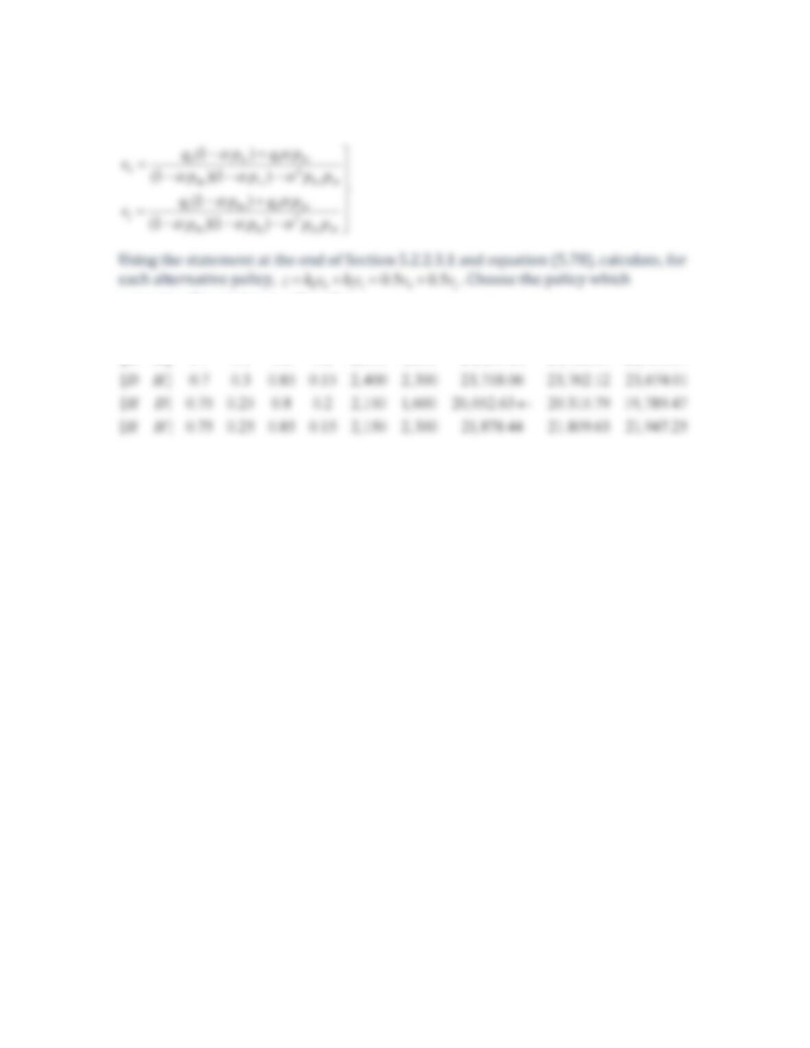
5.10d) To use exhaustive enumeration when α = 0.9, solve the set of VDEs generated by
the MCR which corresponds to each of the 4 alternative policies.
109
The solution for the expected total discounted costs is given by equation (4.264) below.
00 11 0 1
z
Ǥ
00 01 10 11 0 1 0 1
Policy
[ ] 0.7 0.3 0.8 0.2 2,400 1,600 24,367.58 24,780.59 23,954.57
pppp q q z v v
DD