78
5.5)
5.5a)
Reward yProbabilit TransitionDecisionState
,,,
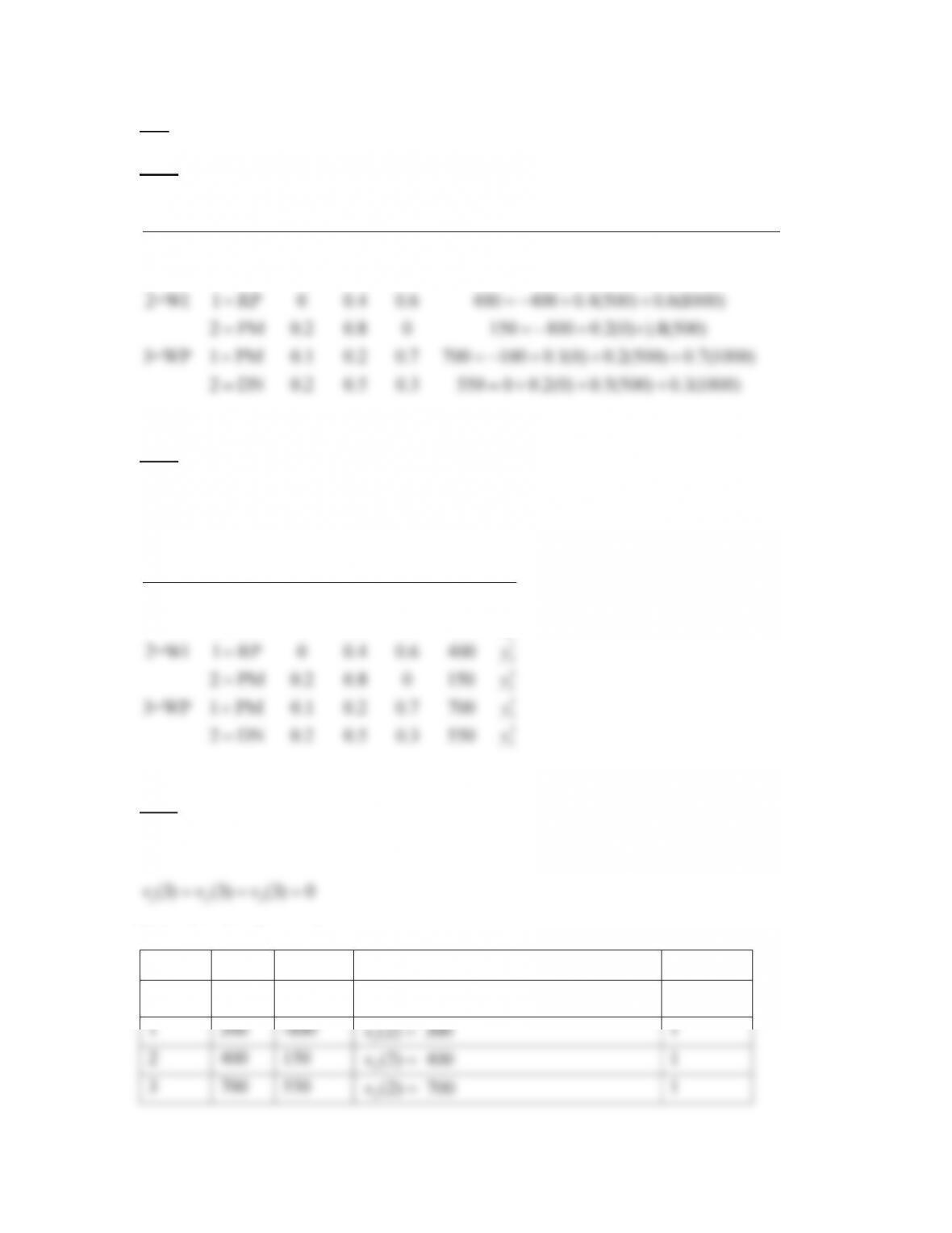
1=NW 1 RP 0.1 0.4 0.5 300 400 0.1(0) 0.4(500) 0.5(1000)
2 RL 0 0 1 600 1600 1000
kkk k
iNW iWI iWP i
ikppp q
2 DN 0.2 0.5 0.3 550 0 0.2(0) 0.5(500) 0.3(1000)
5.5b) The recurrent MDP model of machine maintenance with LP variables added in the
right most column is summarized below.
State Decision Transition Prob. Reward LP
,,,
1
1
2
1
1=NW 1 RP 0.1 0.4 0.5 300
2 RL 0 0 1 600
kkk kk
iNW iWI iWP i i
ikpppqy
y
y
5.5c) To begin value iteration, assume zero expected total rewards are received in every
state at the end of day 3.
123
(3) (3) (3) 0vvv
Value iteration for
2n
State
1
i
q
2
i
q
Expected Total Reward
Decision
i
1 k
2 k
12
(2) max[ , ]
iii
k
vqq
, for
1, 2, 3i
k
1
300
-600
1(2) 300v
1
2
400
150
2(2) 400v
1
3
700
550
3(2) 700v
1
Value iteration for
1n
i
k
123
(300) (400) (700)
kk k k
ii i i
qp p p
(1)
i
v
(1)
i
dk
1
1
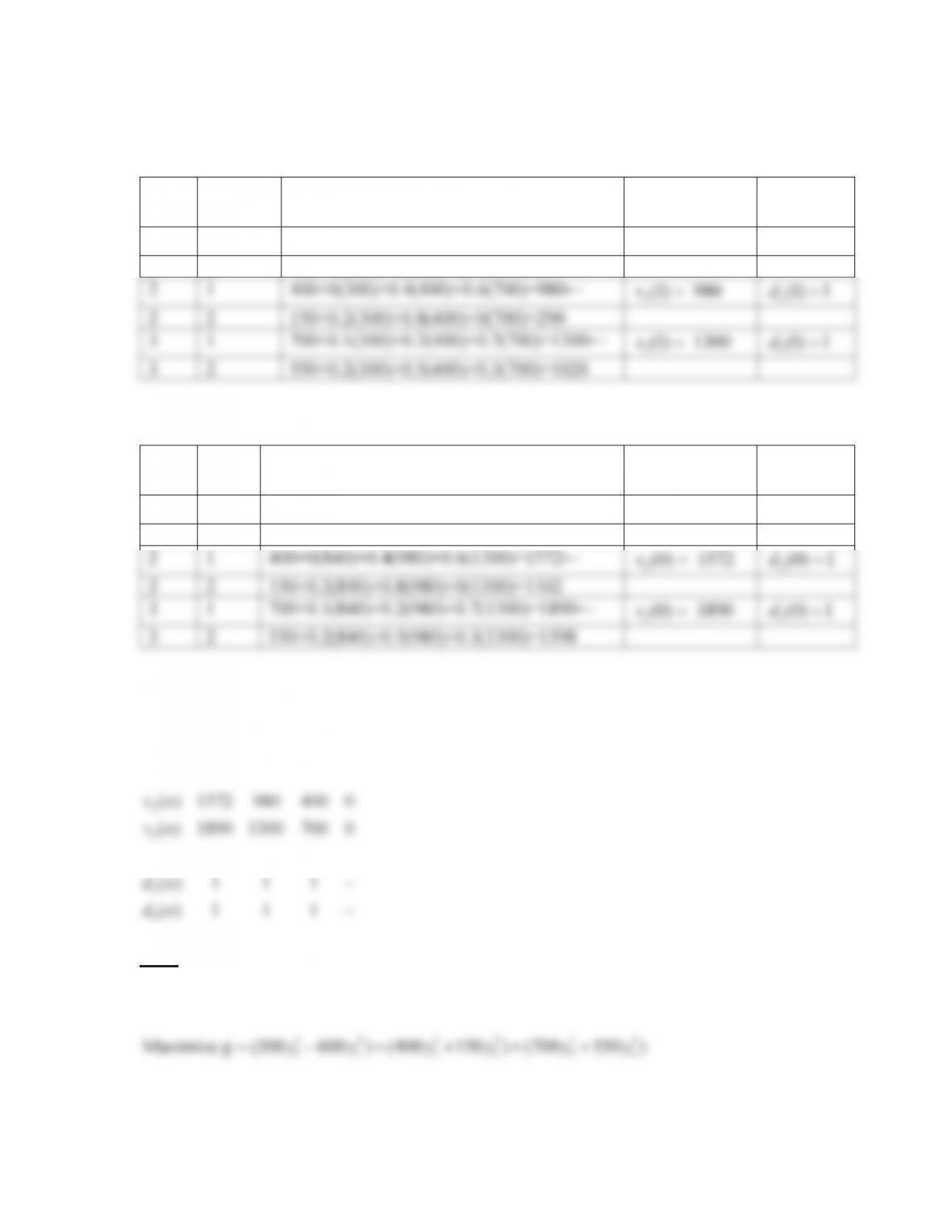
300+0.1(300)+0.4(400)+0.5(700)=840←
1(1) 840v
1
(1) 1d
1
2
-600+0(300)+0(400)+1(700)=100
2
1
400+0(300)+0.4(400)+0.6(700)=980←
2(1) 980v
2
(1) 1d
2
2
150+0.2(300)+0.8(400)+0(700)=290
3
1
700+0.1(300)+0.2(400)+0.7(700)=1300←
(1) 1300v
i
k
1
2
-600+0(840)+0(980)+1(1300)=700
2
1
2
2
3
1
3
2
80
12 1 2 1 2
11 2 2 3 3
1) (0.9 ) (0 0.2 ) ( 0.1 0.2 ) 0yy y y y y
10yt
1
2
2
30yt
3
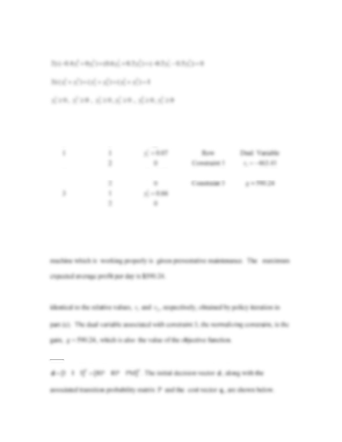
The solution of the recurrent LP model is summarized below.
1
2
Objective function value, g 590.24
2 1 0.27
k
iky
y
1
2
Constraint 2 317.07
v
The optimal policy is given by the vector
[1 1 1] [RP RP PM]
TT
d
. Under this
policy, a machine which is not working or is working intermittently is replaced, and a
The LP solution shows that the dual variables associated with constraints 1 and 2 are
5.5e) To begin policy iteration, arbitrarily choose the initial policy
TT
81
1 0.1 0.4 0.5 300
ªº ª º ª º
¬¼ ¬ ¼ ¬ ¼
The VDEs are
1123
300 0.1 0.4 0.5
gv v v v
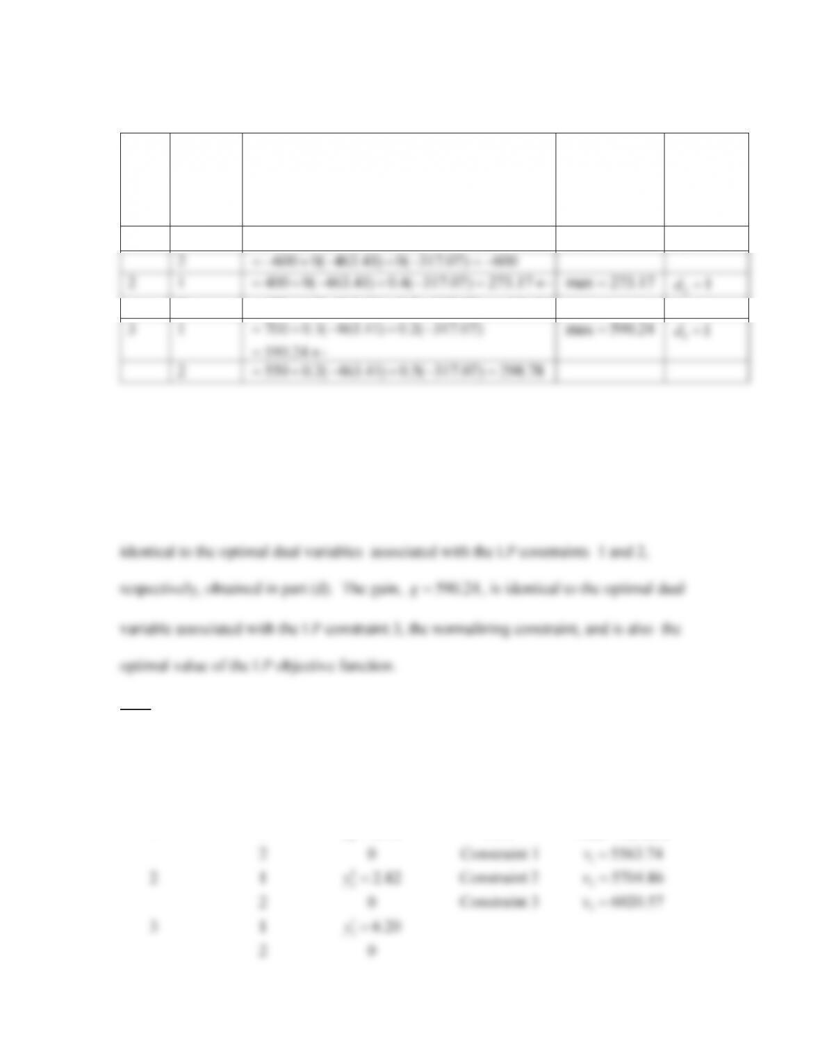
First policy improvement for machine maintenance model
State Decision Test Quantity
State
i
Decision
Alterna-
tive
k
11 2 2 3 3
12 3
Test Quantity
( 463.41) ( 317.07) (0)
kk k k
ii i i
kk k k
ii i i
qpvpvpv
qp p p
Maximum
Value of
Test
Quantity
Decision
kd
i
1
1
300 0.1( 463.41) 0.4( 317.07) 126.83 m
max 126.83
1
1d
2
1
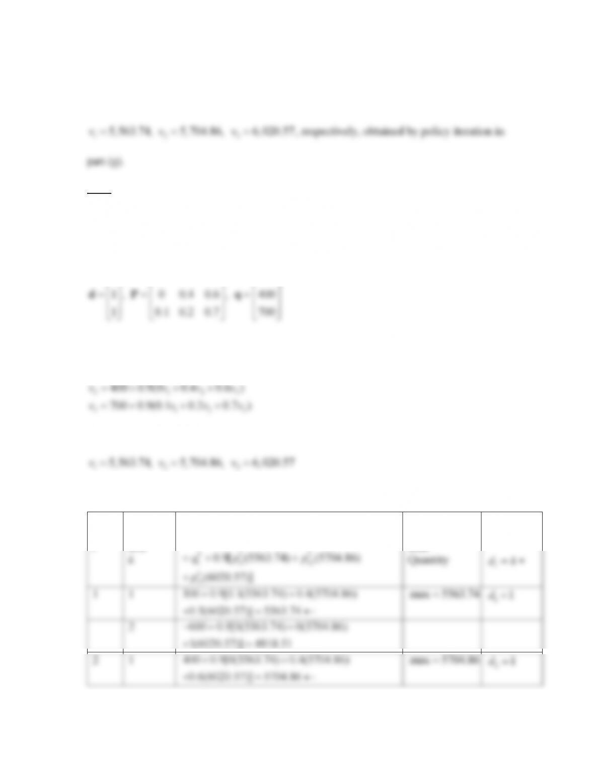
Note that the dual variables associated with LP constraints 1, 2, and 3, respectively, are
identical to the expected total discounted rewards,
5,563.74, 5, 704.86, 6,020.57vv v
, respectively, obtained by policy iteration in
5.5g) Begin policy iteration with
0.9
D
by choosing an initial policy given by the
vector
[1 1 1] [RP RP PM]
TT
d
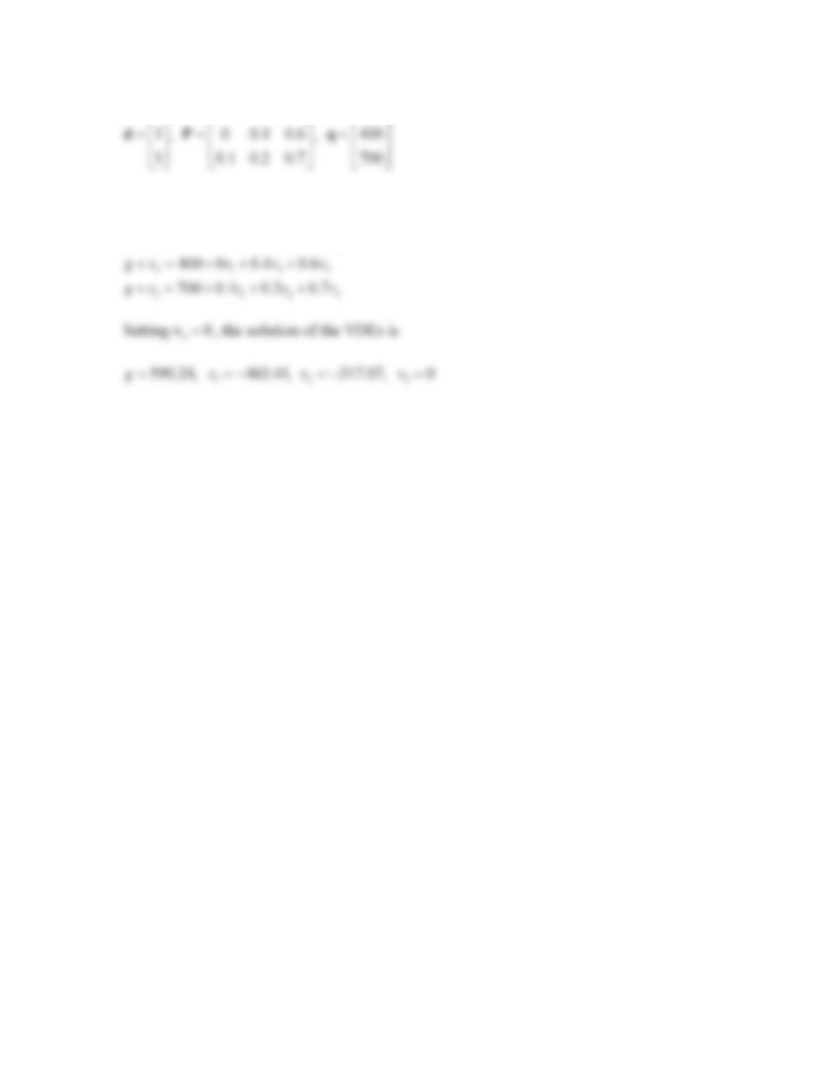
. The initial decision vector
d
, along with the
associated transition probability matrix
P
and the cost vector
q
, are shown below.
1 0.1 0.4 0.5 300
ªº ª º ª º
¬¼ ¬ ¼ ¬ ¼
The VDEs are
1123
300 0.9(0.1 0.4 0.5 )
vvvv
The solution of the VDEs is
12 3
5,563.74, 5, 704.86, 6,020.57vv v
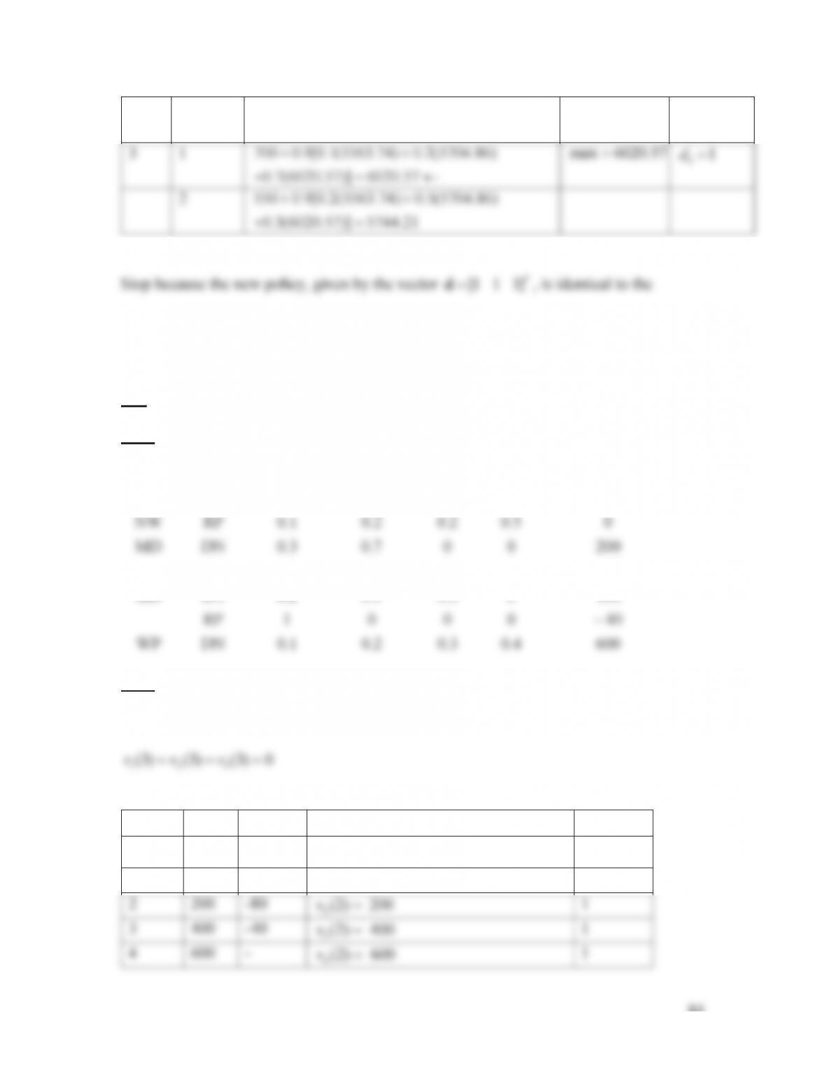
First policy improvement for machine maintenance model
State Decision Test Quantity
State
i
Decision
Alterna-
tive
11 2 2 3 3
Test Quantity
()
kkkk
iiii
qpvpvpv
D
Maximum
Value of
Test
Decision
84
2
150 0.9[0.2(5563.74) 0.8(5704.86)
0(6020.57)] 5258.97
3
1
700 0.9[0.1(5563.74) 0.2(5704.86)
0.7(6020.57)] 6020.57
m
max 6020.57
3
1d
2
550 0.9[0.2(5563.74) 0.5(5704.86)
0.3(6020.57)] 5744.21
T
previous policy. Therefore, this policy is optimal.
5.6)
5.6a)
6004.03.02.01.0DNWP
40003.05.02.0DNmD
800001RP
200007.03.0DNMD
05.02.02.01.0RPNW
WPmDMDNW
Reward ExpectedyP robabilitTransitionActionState
11
k
inn qjjjjkdiX
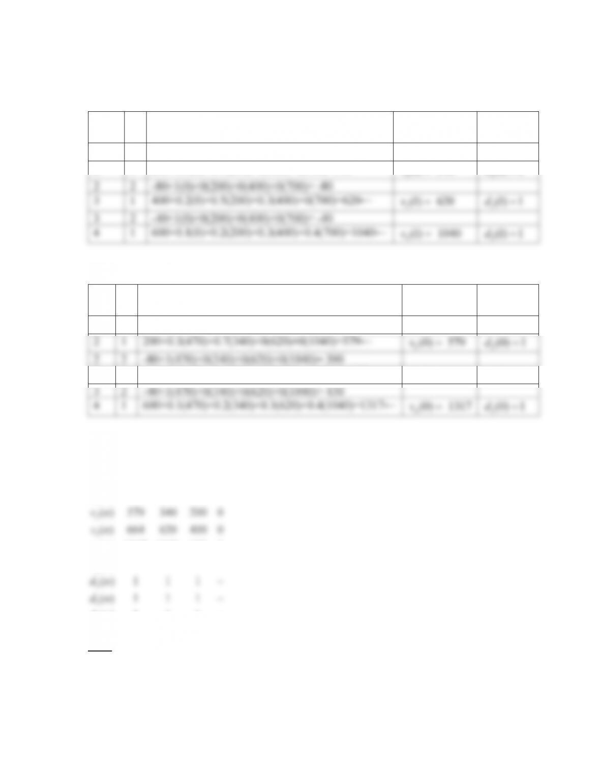
5.6b) To begin value iteration, assume zero expected total rewards are received in every
state at the end of day 3.
123
(3) (3) (3) 0vvv
Value iteration for
2n
State
1
i
q
2
i
q
Expected Total Reward
Decision
i
1 k
2 k
12
(2) max[ , ]
iii
k
vqq
, for
1, 2, 3, 4i
k
1
0
–
1
(2) 0v
1
2
200
-80
2(2) 200v
1
3
400
-40
3(2) 400v
1
4
600
–
4
(2) 600v
1
85
Value iteration for
1n
i
k
1234
(0) (200) (400) (600)
kk k k k
ii i i i
qp p p p
(1)
i
v
(1)
i
dk
1
1
0+0.1(0)+0.2(200)+0.2(400)+0.5(700)=470←
1(1) 470v
1
(1) 1d
2
1
200+0.3(0)+0.7(200)+0(400)+0(700)=340←
(1) 340v
2
2
-80+1(0)+0(200)+0(400)+0(700)= -80
3
1
400+0.2(0)+0.5(200)+0.3(400)+0(700)=620←
(1) 620v
3
2
-40+1(0)+0(200)+0(400)+0(700)= -40
4
1
600+0.1(0)+0.2(200)+0.3(400)+0.4(700)=1040←
4
(1) 1040v
3
(1) 1d
Value iteration for
0n
i
k
1234
(470) (340) (620) (1040)
kk k k k
ii i i i
qp p p p
(0)
i
v
(0)
i
dk
1
1
0+0.1(470)+0.2(340)+0.2(620)+0.5(1040)=759←
1(0) 759v
1(0) 1d
2
1
200+0.3(470)+0.7(340)+0(620)+0(1040)=579←
(0) 579v
2
2
-80+1(470)+0(340)+0(620)+0(1040)= 390
3
1
400+0.2(470)+0.5(340)+0.3(620)+0(1040)=664←
3(0) 664v
3(0) 1d
3
2
-40+1(470)+0(340)+0(620)+0(1040)= 430
4
1
600+0.1(470)+0.2(340)+0.3(620)+0.4(1040)=1317←
An optimal policy over the next three days is summarized below.
1
4
1
4
0123
( ) 759 470 0 0
( ) 1317 1040 600 0
() 1 1 1
() 1 1 1
n
vn
vn
dn
dn
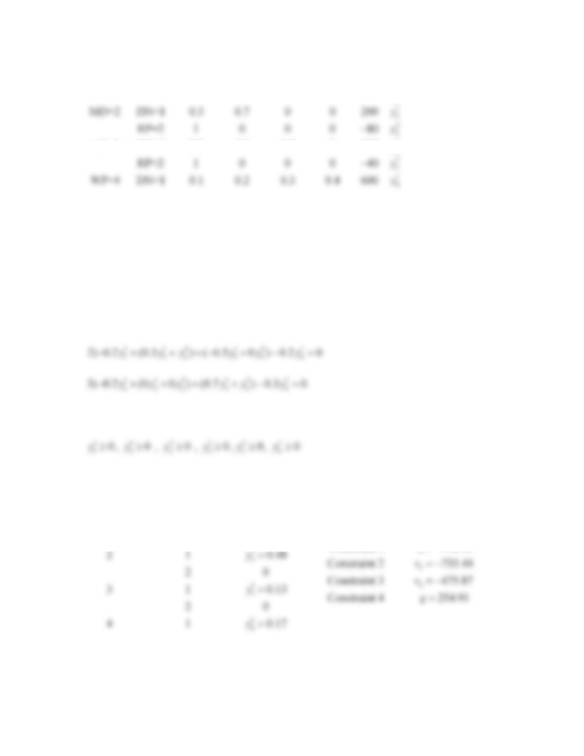
5.6c) The recurrent MDP model of machine repair with LP variables added in the right
most column is summarized below.
86
11
1
1
1
3
1NW2MD3mD4WP
NW=1 RP=1 0.1 0.2 0.2 0.5 0
mD=3 DN=1 0.2 0.5 0.3 0 400
kk
nn ii
Xidk qy
y
y
After omitting the last constraint which is redundant, the linear programming formulation
for the recurrent MDP model of machine repair appears below.
112 121
122 334
Maximize g 0 (200 80 ) (400 40 ) 600yyy yyy
subject to
112 121
122 334
1) 0.9 ( 0.3 ) ( 0.2 ) 0.1 0yyy yyy
112 121
122 334
4) ( ) ( ) 1yyy yyy
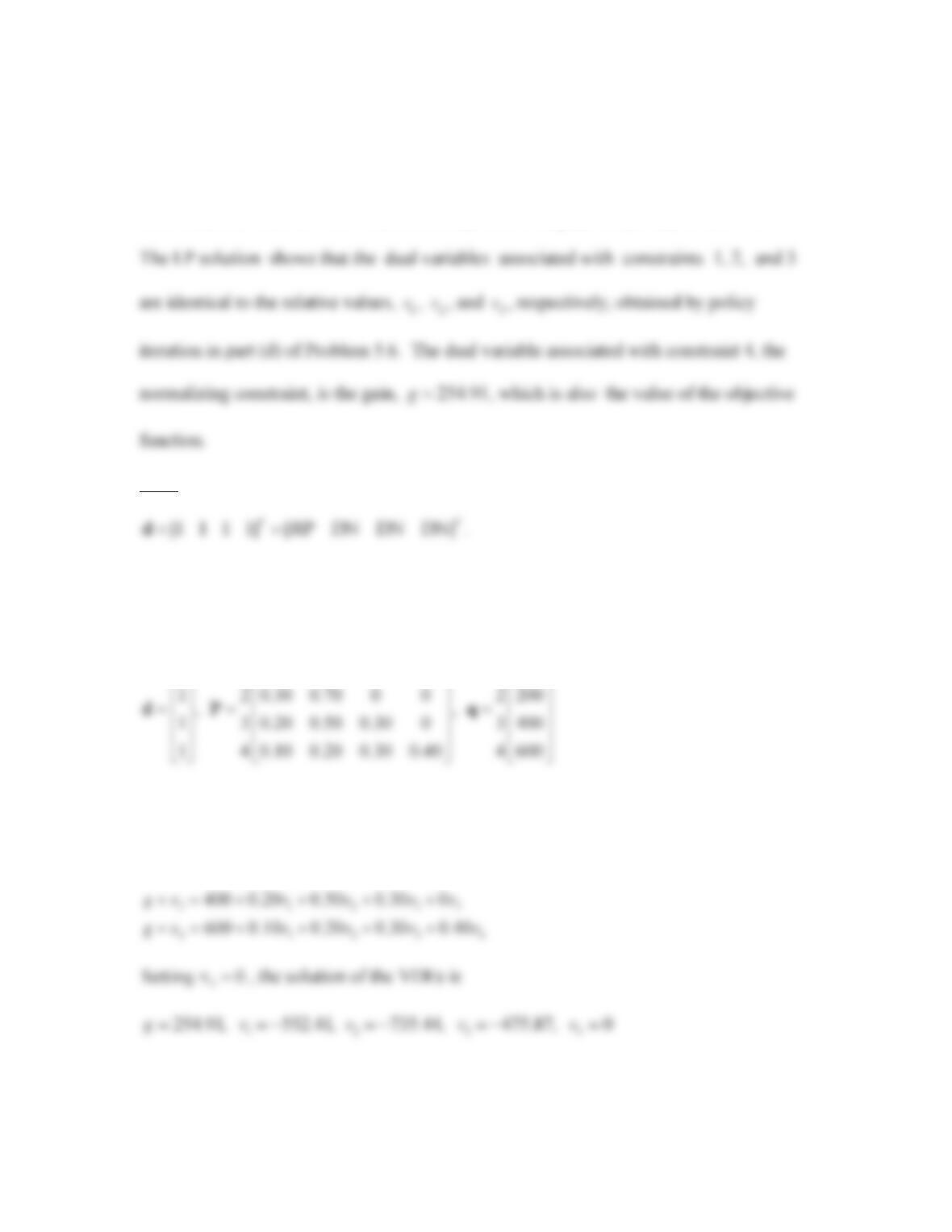
The solution of the recurrent LP model is summarized below.
1
1
Objective function value, g 254.91
1 1 0.21
k
i
iky
y
Row Dual Variable
Constraint 1 552.41
v
87
The optimal policy is given by the vector
[1111] [RP DN DN DN]
TT
d
.
Under this policy, a machine which is not working is repaired, and a machine in every
other state is left alone. The maximum expected average profit per day is $254.91.
5.6d) Begin policy iteration by choosing an initial policy given by the vector
TT
The initial decision vector
d
, along with the associated transition probability matrix
P
and the reward vector
q
, are shown below.
1 1 0.10 0.20 0.20 0.50 1 0
ªº ª º ª º
¬¼ ¬ ¼ ¬ ¼
The VDEs are
1 1234
2 1 234
0 0.10 0.20 0.20 0.50
200 0.30 0.70 0 0
gv v v v v
gv v v v v
12 3 4
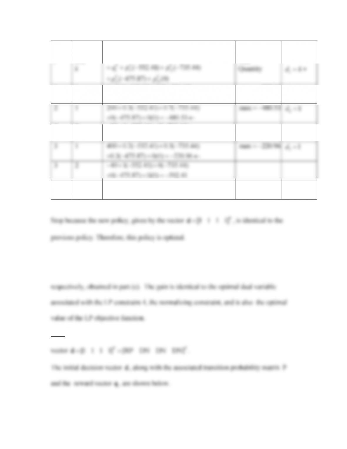
First policy improvement for machine repair model
State Decision Test Quantity
State
i
Decision
Alterna-
tive
11 22 33 44
Test Quantity
kk k k k
ii i i i
qpvpvpvpv
Maximum
Value of
Test
Decision
89
1 1 0.10 0.20 0.20 0.50 1 0
ªº ª º ª º
¬¼ ¬ ¼ ¬ ¼
The VDEs are
1 1234
0 0.9(0.10 0.20 0.20 0.50 )
vvvvv
The solution of the VDEs is
12 3 4
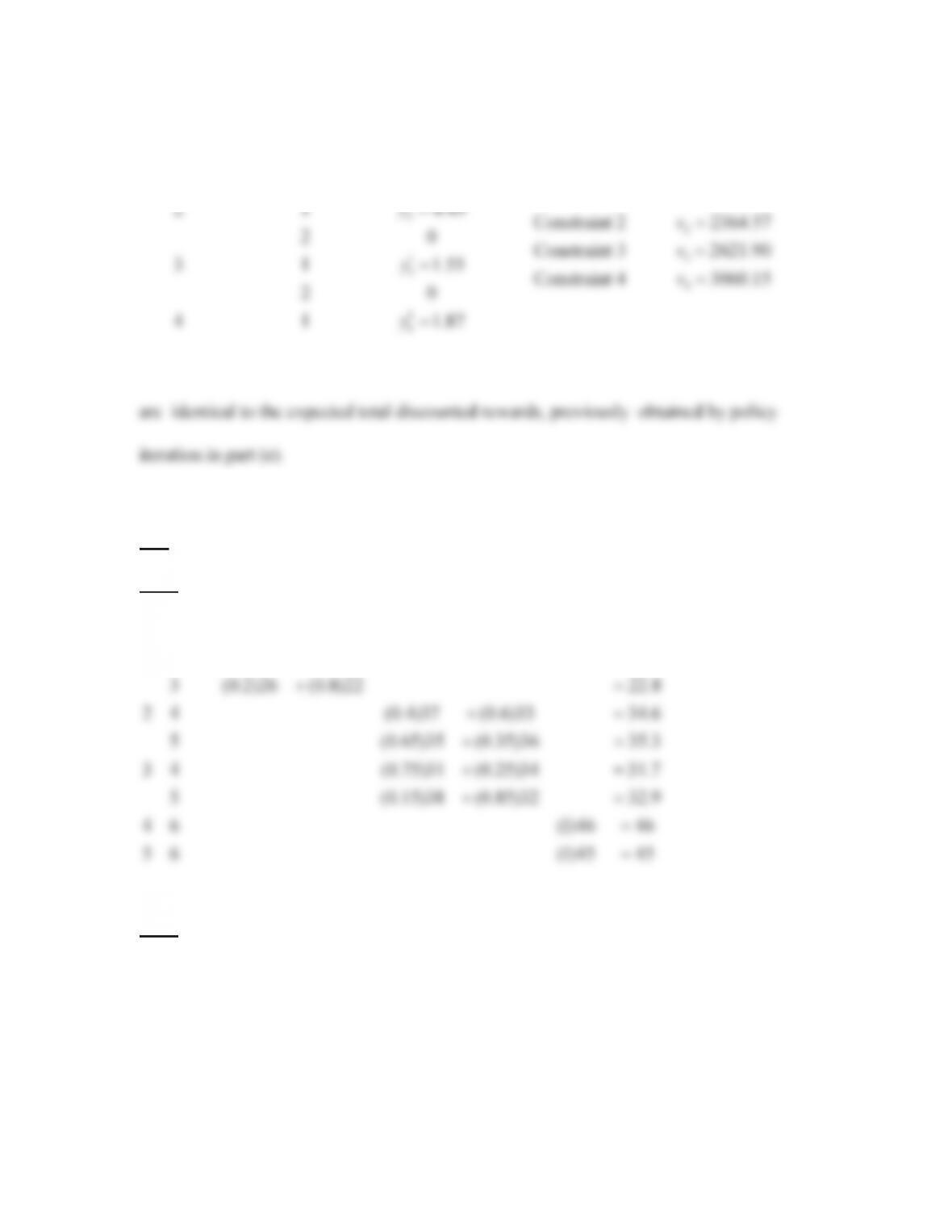
2499.60, 2364.57, 2621.90, and 3060.15vv v v
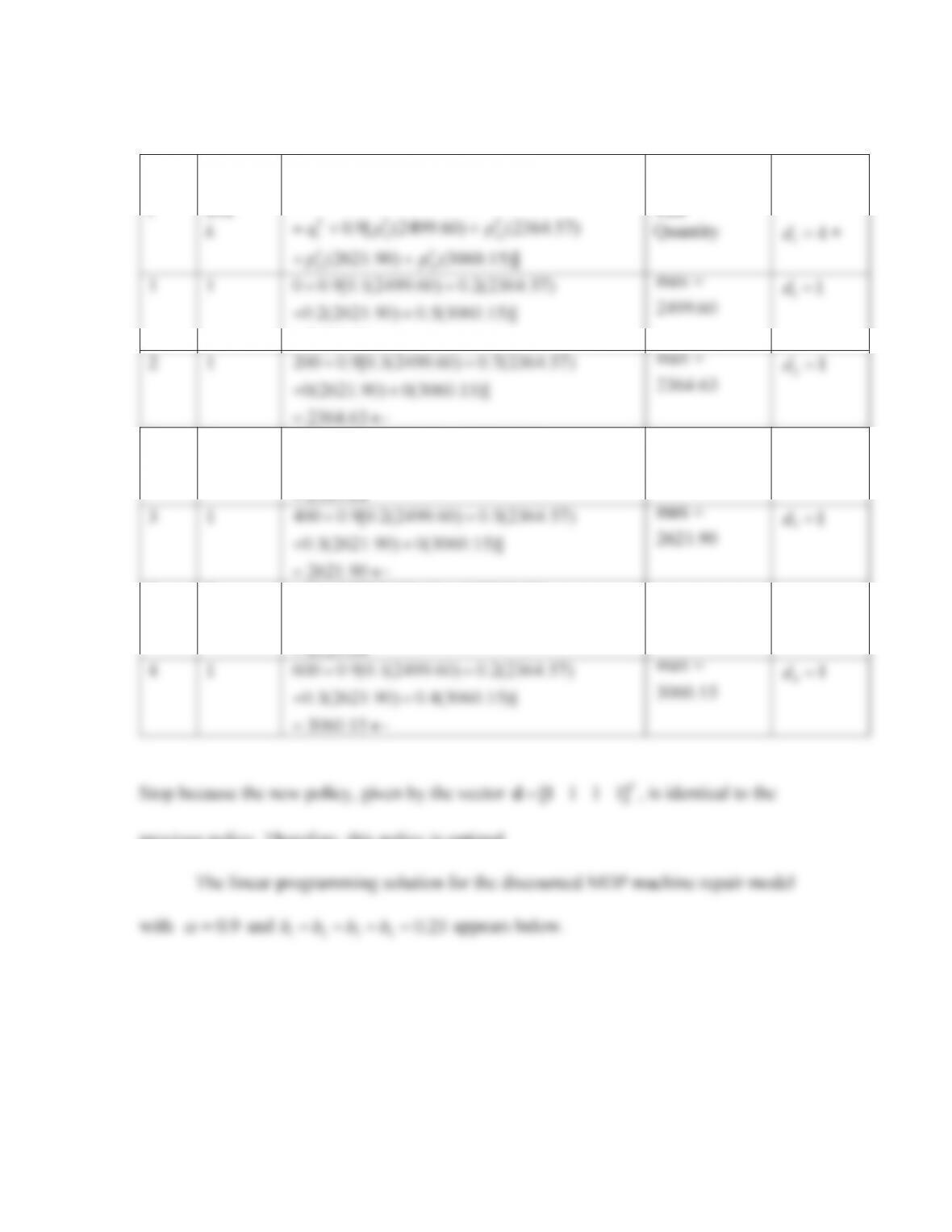
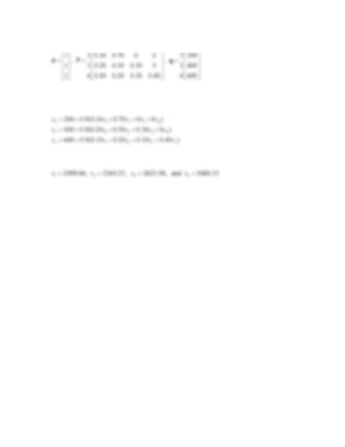
First policy improvement for machine repair model
State Decision Test Quantity
State
i
Decision
Alterna-
tive
11 22 33 44
Test Quantity
()
kkkkk
iiiii
qpvpvpvpv
D
Maximum
Value of
Test
Decision
91
1
1
1
Objective function value, z 2636.55
1 1 2.10
k
i
iky
y
1
Row Dual Variable
Constraint 1 2499.60
v
Note that the dual variables associated with LP constraints 1, 2, 3, and 4, respectively,
5.7)
5.7a)
4545)1(65
4646)1(64
9.3232)85.0(38)15.0(5
7.3134)25.0(31)75.0(43
3.3536)35.0(35)65.0(5
6.3433)6.0(37)4.0(42
8.2222)8.0(26)2.0(3
6.2325)
3.0(23)7.0(21
6655443322
k
i
k
i
k
i
k
i
k
i
k
i
k
i
k
i
k
i
k
i
k
i
qrprprprprpki
5.7b)
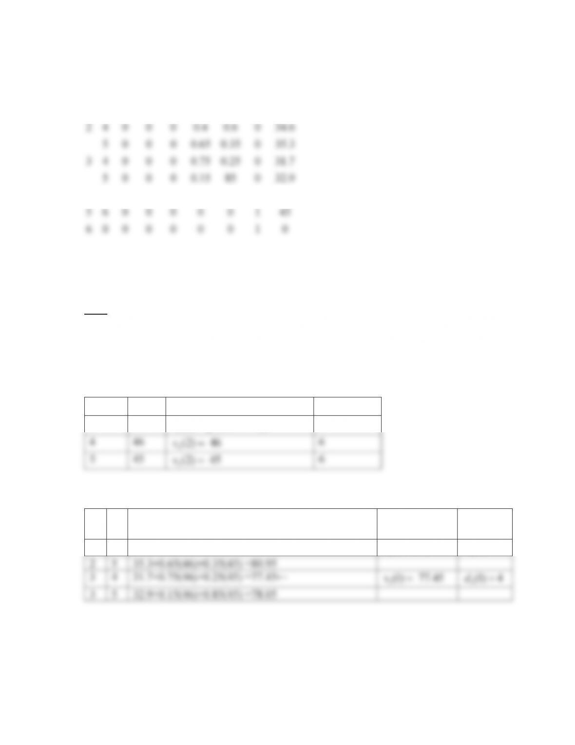
92
1234 56
1 2 0 0.7 0.3 0 0 0 23.6
3 0 0.2 0.8 0 0 0 22.8
46 0 0 0 0 0 1 46
kk k k k k k
ii i i i i i
ikp p p p p p q
The stochastic shortest route model is a unichain MDP because node 6 is an absorbing
state.
5.7c) To begin value iteration at the end of day 3, specify zero expected total distance
from node 6 to the final destination.
6(3) 0v
Value iteration for
2n
State
6
i
q
Expected Total Distance
Decision
i
6k
6
(2)
ii
vq
, for
4,5i
k
4
46
4
(2) 46v
6
5
45
5
(2) 45v
6
Value iteration for
1n
i
k
45
(46) (45)
kk k
ii i
qp p
(1)
i
v
(1)
i
dk
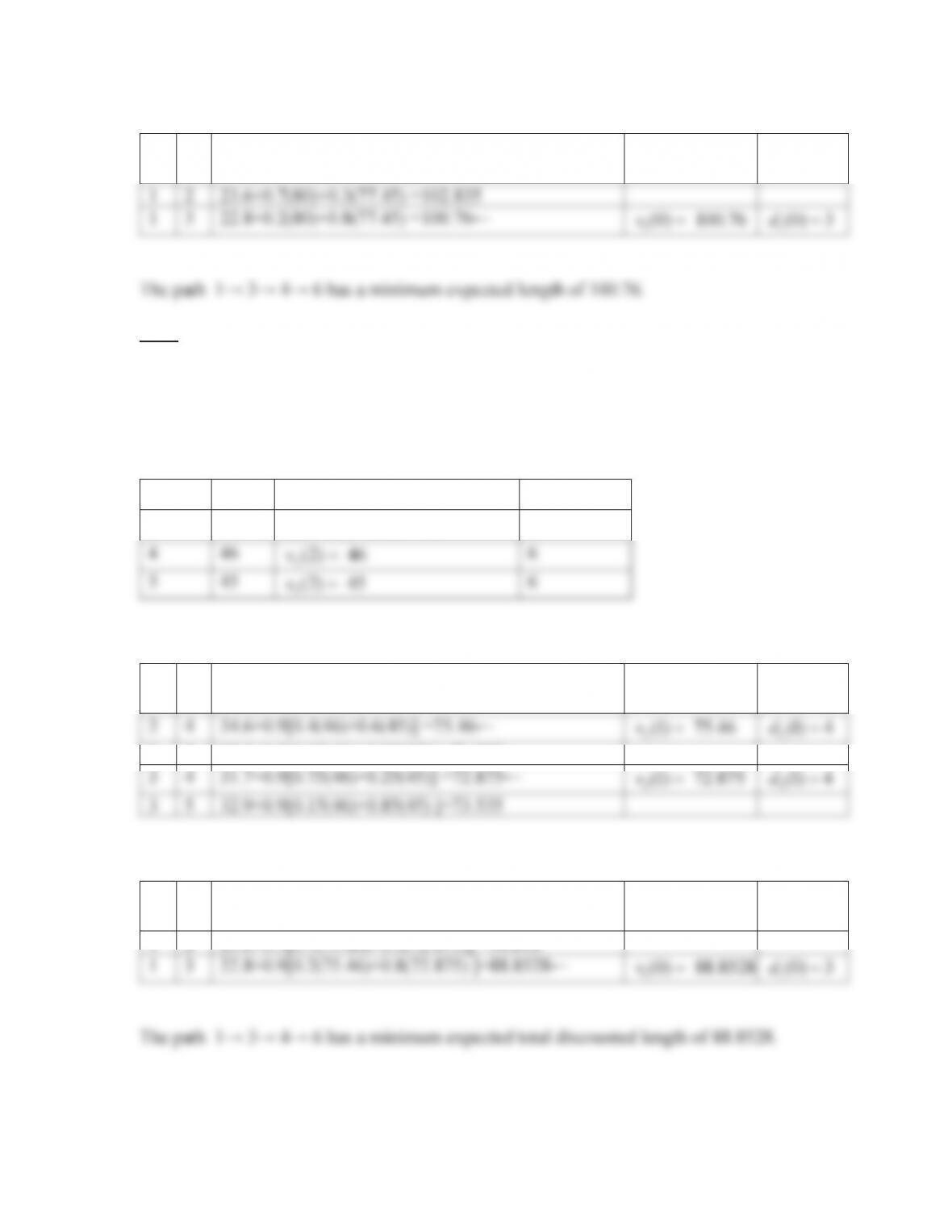
2
4
34.6+0.4(46)+0.6(45) =80←
2
(1) 80v
2(1) 4d
2
5
35.3+0.65(46)+0.35(45) =80.95
3
4
31.7+0.75(46)+0.25(45) =77.45←
3(1) 77.45v
3(1) 4d
3
5
32.9+0.15(46)+0.85(45) =78.05
93
Value iteration for
0n
i
k
23
(80) (77.45)
kk k
ii i
qp p
(0)
i
v
(0)
i
dk
1
2
23.6+0.7(80)+0.3(77.45) =102.835
1
3
22.8+0.2(80)+0.8(77.45) =100.76←
1
(0) 100.76v
1
(0) 3d
5.7d) Value iteration, using a discount factor of
9.0
D
, begins at the end of day 3.
Specify a zero expected total discounted distance from node 6 to the final destination.
6(3) 0v
Value iteration for
2n
State
6
i
q
Expected Total Distance
Decision
i
6k
6
(2)
ii
vq
, for
4,5i
k
4
46
4
(2) 46v
6
5
45
5
(2) 45v
6
Value iteration for
1n
i
k
45
[ (46) (45)]
kk k
ii i
qp p
D
(1)
i
v
(1)
i
dk
2
4
34.6+0.9[0.4(46)+0.6(45)] =75.46←
2
(1) 75.46v
2(1) 4d
2
5
35.3+0.9[0.65(46)+0.35(45)] =76.385
3
4
31.7+0.9[0.75(46)+0.25(45)] =72.875←
3(1) 72.875v
3
(1) 4d
3
5
32.9+0.9[0.15(46)+0.85(45) ]=73.535
Value iteration for
0n
i
k
23
[ (75.46) (72.875)]
kk k
ii i
qp p
D
(0)
i
v
(0)
i
dk
1
2
23.6+0.9[0.7(75.46)+0.3(72.875)] =90.816
1
3
22.8+0.9[0.2(75.46)+0.8(72.875) ]=88.8528←
1(0) 88.8528v
1
(0) 3d