58
CHAPTER 5 A MARKOV DECISION PROCESS (MDP)
5.1)
5.1a) The bidding problem will be formulated as a unichain MDP and solved by value
iteration over a 4-week planning horizon. To formulate the problem as an MDP, note that
there are two decisions: to accept (decision A) or reject (decision R) the
thn
offer. There
n
the bidding problem is shown in the table below.
RewardyProbabilit TransitionDecisionState
,16 ,18 ,22 ,24 ,
16 1 A 0 0 0 0 1 16
22 1 A 0 0 0 0 1 22
2 R 0.4 0.1 0.3 0.2 0 0
kkkk kk
iiiiii
ikpppppq
‘
5.1b) Value iteration begins at the end of the planning horizon, at the end of week 4. For
4 n
,
4
i
59
16
18
22
24
The calculations for week 3, denoted by
3 n
, are indicated below.
,22,2418,16for ,]}reject if )24(2.0)22(3.0)18(1.0)16(4.0[ accept], if {[max)3(
,22,2418,16for
,]}reject if )4(2.0)4(3.0)4(1.0)4(4.0[ accept], if {[max)3(
3
242218163
ixv
i
vvvvxv
i
i
accept ,24}reject] if 6.19[ accept], if 24{[max)3( then ,24 If
accept 22,}reject] if 6.19[ accept], if 22{[max)3( then ,22 If
243
223
183
viX
viX
The calculations for week 2, denoted by
2 n
, are indicated below.
22,24,18,16for ,}reject] if 2.21[ accept], if {[max)2(
,22,2418,16for ,]}reject if )24(2.0)22(3.0)6.19(1.0)6.19(4.0[ accept], if {[max)2(
,22,2418,16for
,]}reject if )3(2.0)3(3.0
)3(1.0)3(4.0[ accept], if {[max)2(
2
2
242218162
ixv
ixv
i
vvvvxv
i
i
i
accept ,24}reject] if 2.21[ accept], if 24{[max)2( then ,24 If
accept 22,}reject] if 2.21[ accept], if 22{[max)2( then ,22 If
reject ,2.21}reject] if 2.21[ accept], if 18{[max)2( then 18, If
reject ,2.21}reject] if 2.21
[ accept], if 16{[max)2( then 16, If
242
222
182
162
viX
viX
viX
viX
Finally, the calculations for week 1, denoted by
1 n
, are indicated below.
60
22,24,18,16for ,}reject] if 22[ accept], if {[max)1(
,22,2418,16for ,]}reject if )24(2.0)22(3.0)2.21(1.0)2.21(4.0[ accept], if {[max)1(
,22,2418,16for
,]}reject if )2(2.0)2(3.0)2
(1.0)2(4.0[ accept], if {[max)1(
1
1
242218161
ixv
ixv
i
vvvvxv
i
i
i
accept ,24}reject] if 22[ accept], if 24{[max)1( then ,24 If
rejector accept 22,}reject] if 22[ accept], if 22{[max)1( then ,22 If
reject ,22}reject] if 22[ accept], if 18{[max)1( then 18, If
reject ,22}reject] if 22[ accept], if 16{[max)
1( then 16, If
241
221
181
161
viX
viX
viX
viX
The results of these calculations are summarized in the form of decision rules given
in the table below.
Continue61Accept then24,or 22, 18, 16, If4
Stop.619Accept then24,or 22 If
ContinueReject then18,or 16 If3
Stop21.2Accept then24,or 22 If
ContinueReject then18,or 16 If2
Stop22Accept then24,or 22 If
ContinueReject then22,or 18, 16, If1
will
Offers
accepted becan
hoffer whic Minimum
Decision Offer, Week,
44
33
3
22
2
11
1
t
!
!
t
XX
XX
X
XX
X
XX
X
Xn n
5.2)
5.2a) Treat this problem as an optimal stopping problem by augmenting the state space
with an absorbing state Δ that is reached with probability 1 when the stock is sold and with
61
2
1
2
20
1
2
15
1
15
2
10
1
2
5
1
5
2
0
1
0
,20,15,10,5,0,
0100000H2
0100000S1
1014.022.038.018.008.0H2
20100000S120
1006.024.040.020.010.0H2
15100000S115
10100000S110
1008.020.032.028.012.0H2
5100000S15
1018.010.026.012.034.0H2
0100000S10
‘
‘
‘
y
y
y
y
y
y
y
y
y
y
y
yqppppppki k
i
k
i
i
i
k
i
k
i
k
i
k
i
k
i
5.2b) The LP formulation with
0.9
D
for the discounted MDP model for deciding
when to sell a stock over an infinite planning horizon is
2
15
1
15
2
10
1
10
2
5
1
5
2
0
1
0
20
1
20 yy
subject to
1)
2.0)072.0()09.0()198.0()108.0()694.0( 2
20
2
15
2
10
2
5
2
0
1
0 yyyyyy
2
2
2
1
2
20
15
10
10
5
0 yyyyyy
4)
2.0)198.0()784.0()126.0()18.0()09.0(
2
20
2
15
1
15
2
10
2
5
2
0
yyyyyy
1
2
2
2
2
0ty
0ty
5ty
5ty
10 ty
10 ty
15
15 ty
20
20
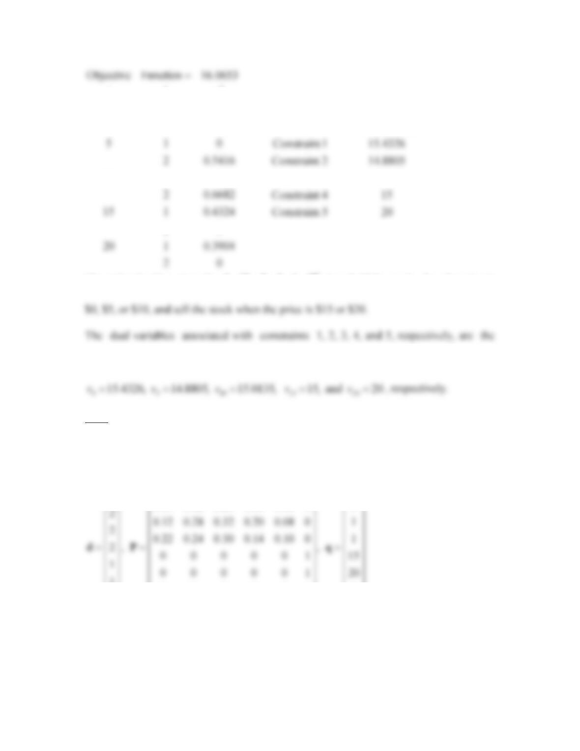
The solution of the LP model for deciding when to sell a stock is summarized below.
62
02
3904.0120
02
4324.0115
6682.02
0110
5416.02
015
5631.02
010
k
i
yki
205 Constraint
154 Constraint
0135.153 Constraint
8805.142 Constraint
4326.151 Constraint
Variable DualRow
The optimal policy, given by
T
]11222[ d
, is to hold the stock when the price is
expected total discounted rewards,
5.2c) Begin policy iteration with
0.9
D
by choosing an initial policy given by the
vector
T
]11222[ d
. The initial decision vector
d
, along with the associated
transition probability matrix
P
and the cost vector
q
, are shown below.
0.34 0.12 0.26 0.10 0.18 0 1
1000001 0
ªºªº
«» «»«»
¬¼ ¬¼¬¼
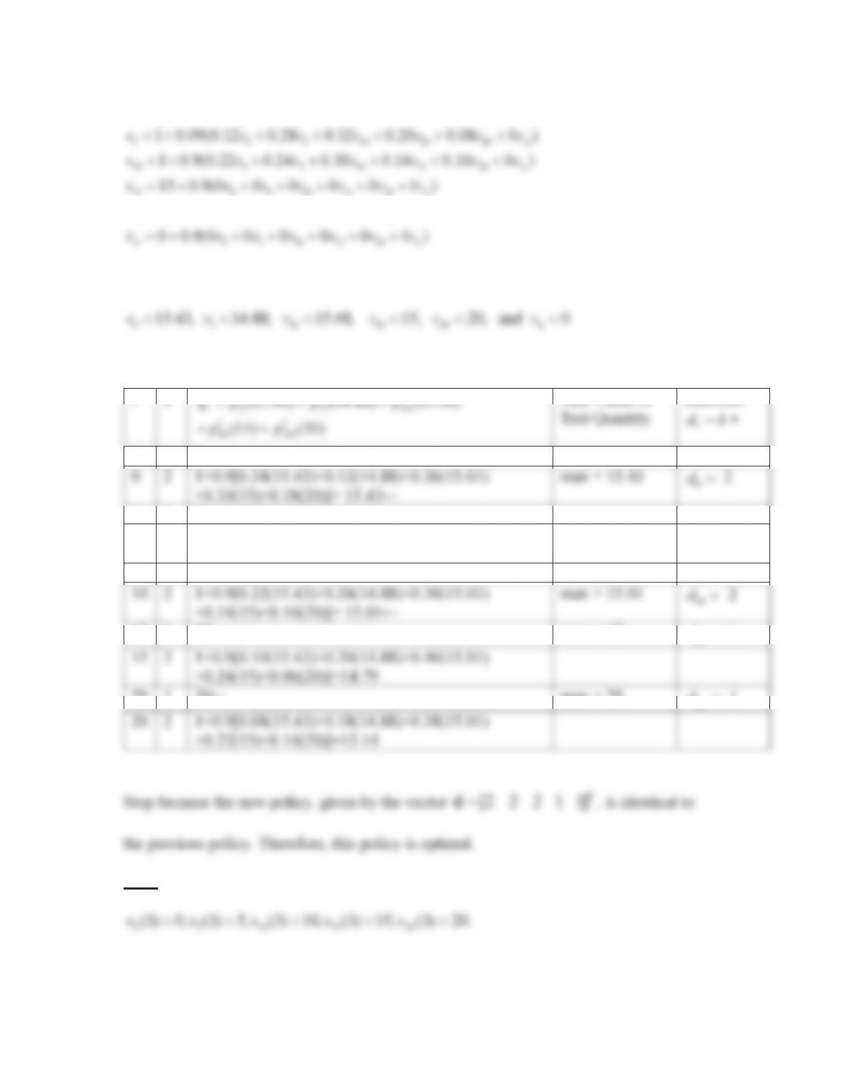
The VDEs are
005101520
20
1 0.9(0.34 0.12 0.26 0.10 0.18 0 )
20
vvvvvvv
v
‘
0 5 10 15 20
0.9(0 0 0 0 0 1 )
vvv v v v
‘
The solution of the VDEs is
0 5 10 15 20
15.43, 14.88, 15.01, 15, 20, and 0vv v vv v
‘
First policy improvement
State Decision Value Test Quantity
i
k
(15.43) (14.88) (15.01)
kk k k
qppp
Max Value of
Decision
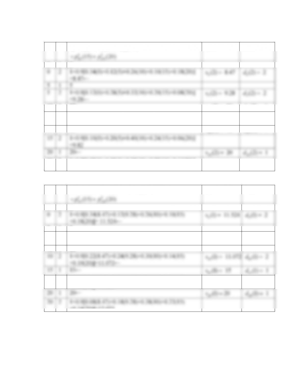
Value iteration for
2n
i
k
0510
(0) (5) (10)
kk k k
ii i i
qp p p
(2)
i
v
(2)
i
dk
0
1
0
0
2
1+0.9[0.34(0)+0.12(5)+0.26(10)+0.10(15)+0.18(20)]
=8.47←
0
(2) 8.47v
0(2) 2d
5
1
5
5
2
1+0.9[0.12(0)+0.28(5)+0.32(10)+0.20(15)+0.08(20)]
=9.28←
5
(2) 9.28v
5
(2) 2d
10
1
10←
10 (2) 10v
10
(2) 1d
10
2
1+0.9[0.22(0)+0.24(5)+0.30(10)+0.14(15)+0.10(20)]
=8.47
15
1
15←
(2) 15v
(2) 1d
15
2
1+0.9[0.10(0)+0.20(5)+0.40(10)+0.24(15)+0.06(20)]
=9.82
20
1
20←
20
(2) 20v
20
(2) 1d
20
2
1+0.9[0.08(0)+0.18(5)+0.38(10)+0.22(15)+0.14(20)]
=9.91
Value iteration for
1n
i
k
0510
(8.47) (9.28) (10)
kk k k
ii i i
qp p p
(1)
i
v
(1)
i
dk
0
1
0
0
2
1+0.9[0.34(8.47)+0.12(9.28)+0.26(10)+0.10(15)
+0.18(20)]= 11.524←
0(1) 11.524v
0
(1) 2d
5
1
5
5
2
1+0.9[0.12(8.47)+0.28(9.28)+0.32(10)+0.20(15)
+0.08(20)]=11.273←
5
(1) 11.273v
5
(1) 2d
10
1
10
10
2
1+0.9[0.22(8.47)+0.24(9.28)+0.30(10)+0.14(15)
+0.10(20)]=11.072←
15
1
15←
(1) 11.072v
15
15
15
2
1+0.9[0.10(8.47)+0.20(9.28)+0.40(10)+0.24(15)
+0.06(20)]=11.353
20
1
20←
(1) 20v
20
2
1+0.9[0.08(8.47)+0.18(9.28)+0.38(10)+0.22(15)
+0.14(20)]=12.023
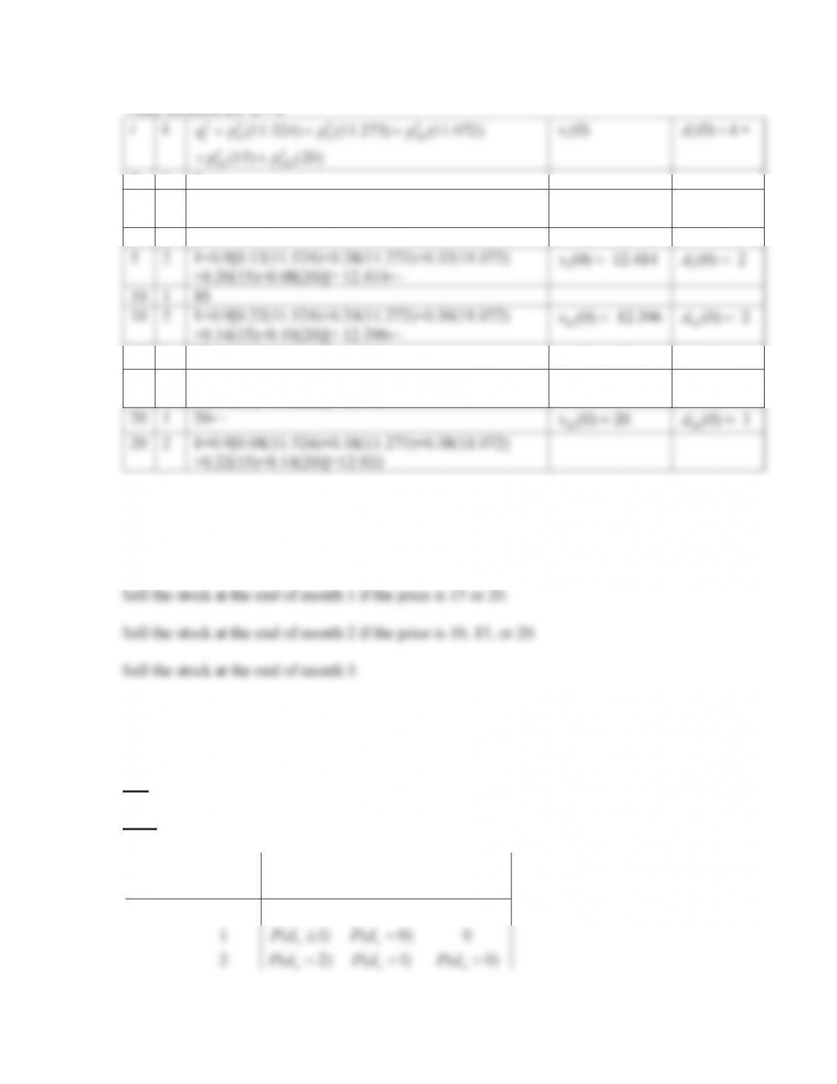
Value iteration for
0n
i
k
0510
15 20
(11.524) (11.273) (11.072)
(15) (20)
kk k k
ii i i
kk
ii
qp p p
pp
(0)
i
v
(0)
i
dk
0
1
0
0
2
1+0.9[0.34(11.524)+0.12(11.273)+0.26(11.072)
+0.10(15)+0.18(20)]= 12.925←
0
(0) 12.925v
0
(0) 2d
5
1
5
5
2
1+0.9[0.12(11.524)+0.28(11.273)+0.32(11.072)
+0.20(15)+0.08(20)]= 12.414←
5
(0) 12.414v
5
(0) 2d
10
1
10
10
2
1+0.9[0.22(11.524)+0.24(11.273)+0.30(11.072)
(0) 12.396v
+0.14(15)+0.10(20)]= 12.396←
20
2
1+0.9[0.08(11.524)+0.18(11.273)+0.38(11.072)
+0.22(15)+0.14(20)]=12.933
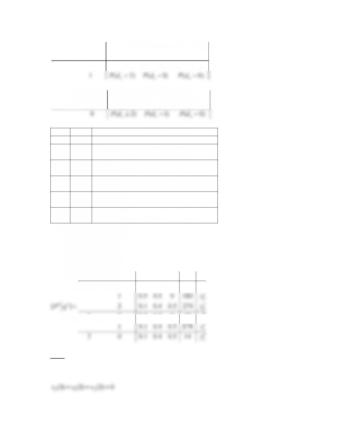
66
1 1 10 11 12
State Decision Transition Probability
1
0(1)(0)0
kk k
nn
nn
Xckp p p
Pd Pd
t
1 1 20 21 22
State Decision Transition Probability
2
kk k
nn
Xckp p p
State
Order
Cost
0
0
$180E(d)=$180(0.6)=$108
1
$60+$100(1)+$180(1)P(d=2)+$10(1)P(d=0)
=60+100(1)+180(0.1)+10(0.5)=$183
2
$60+$100(2) +$10[(2)P(d=0)+(1)P(d=1)]
60+100(2)+10[(2)(0.5)+(1)0.4]=$274
1
0
$180(1)P(d=2)+$10(1)P(d=0)
=180(1)(0.1)+10(0.5)=$23
1
$60+$100(1) +$10[(2)P(d=0)+(1)P(d=1)]
=60+100(1)+10[2(0.5)+1(0.4)]=$174
2
0
$10[(2)P(d=0)+(1)P(d=1)]
=10[2(0.5)+1(0.4)]=$14
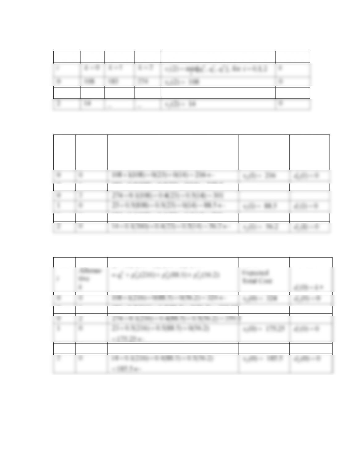
The unichain MDP model of the inventory system with LP variables added in the right
hand column is summarized below.
012
0
0
State Order
0 0 1 0 0 108
kkk kk
iii ii
ikpppqy
y
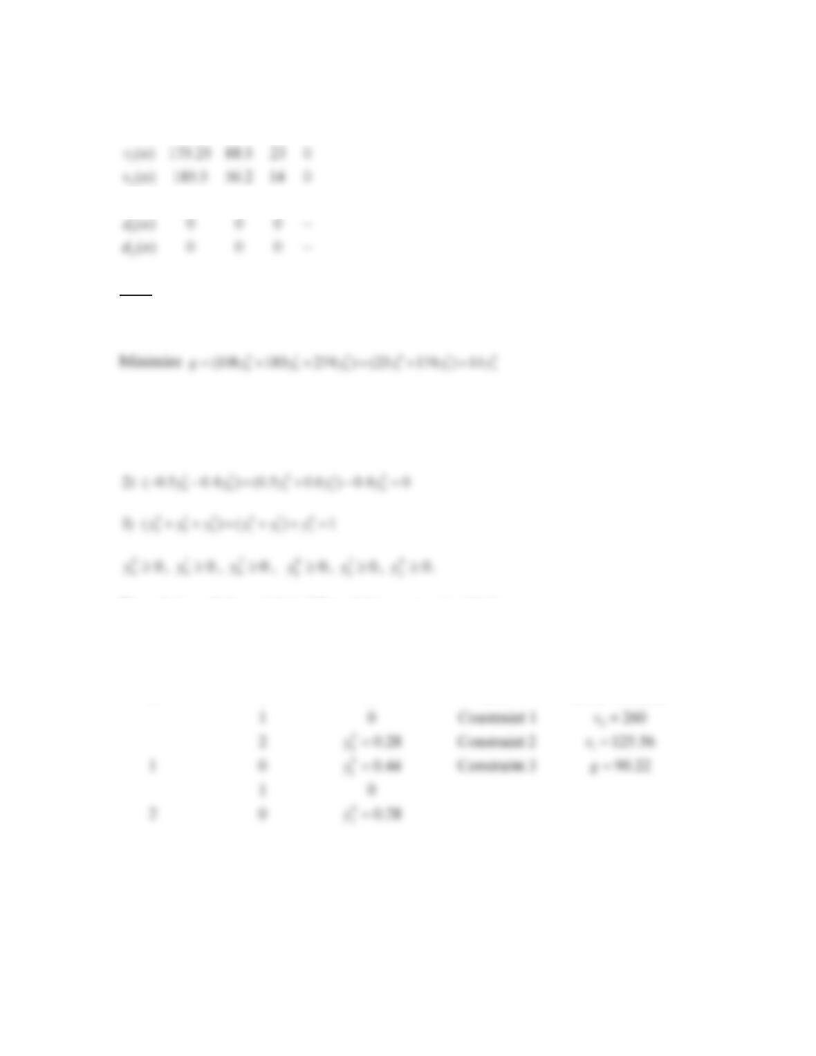
5.3b) To begin value iteration, assume zero expected total costs are received in every
state at the end of day 3.
012
(3) (3) (3) 0vvv
Value iteration for
2n
State
0
i
q
1
i
q
2
i
q
Expected Total Cost
Decision
i
0k
1 k
2 k
012
(2) min[ , , ]
iiii
k
vqqq
, for
0,1, 2i
k
0
108
183
274
0
1
23
174
_
0
2
14
_
_
0
1
0
0
0
68
0
0
0123
( ) 324 216 108 0
() 0 0 0
n
vn
dn
5.3c) After omitting the last constraint which is redundant, the linear programming
formulation for the unichain MDP inventory model appears below.
01 2 010
00 0 112
subject to
12 01 0
00 11 2
1) (0.5 0.9 ) (0.5 0.1 ) 0.1 0yy yy y
0ty
0ty
0ty
1
1
2
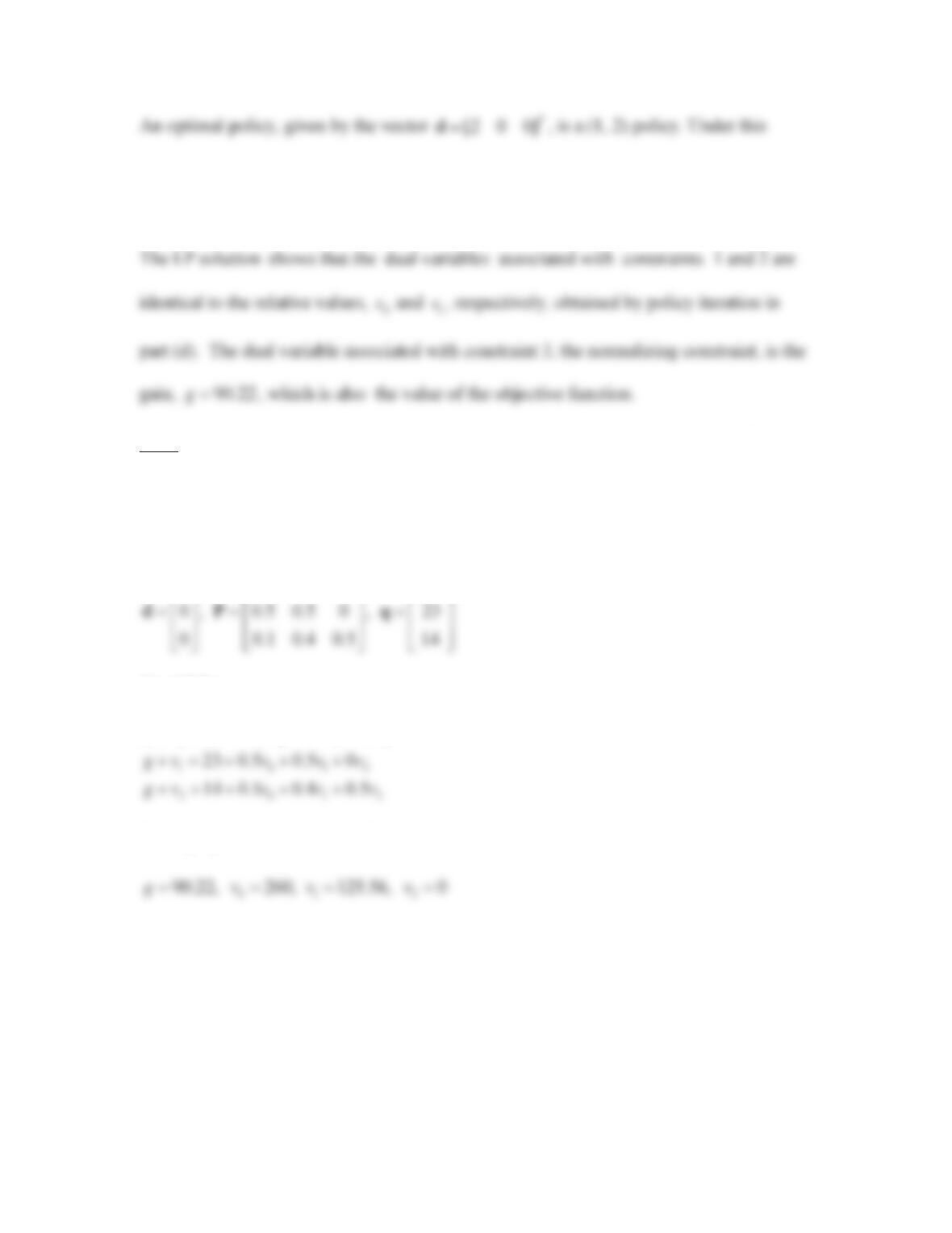
The solution of the unichain LP model is summarized below.
Objective function value, g 90.22
000
k
i
iky
Row Dual Variable
69
T
policy, 2 TVs are ordered when the beginning inventory level is 0; otherwise, no TVs are
ordered. The retailer’s minimum expected average cost per day is $90.22.
5.3d) To begin policy iteration, arbitrarily choose the initial policy
[200]
T
d
. The
initial decision vector
d
, along with the associated transition probability matrix
P
and
the cost vector
q
, are shown below.
2 0.1 0.4 0.5 274
ªº ª º ª º
¬¼ ¬ ¼ ¬ ¼
The VDEs are
0012
274 0.1 0.4 0.5
gv v v v
2
Setting v 0
, the solution of the VDEs is
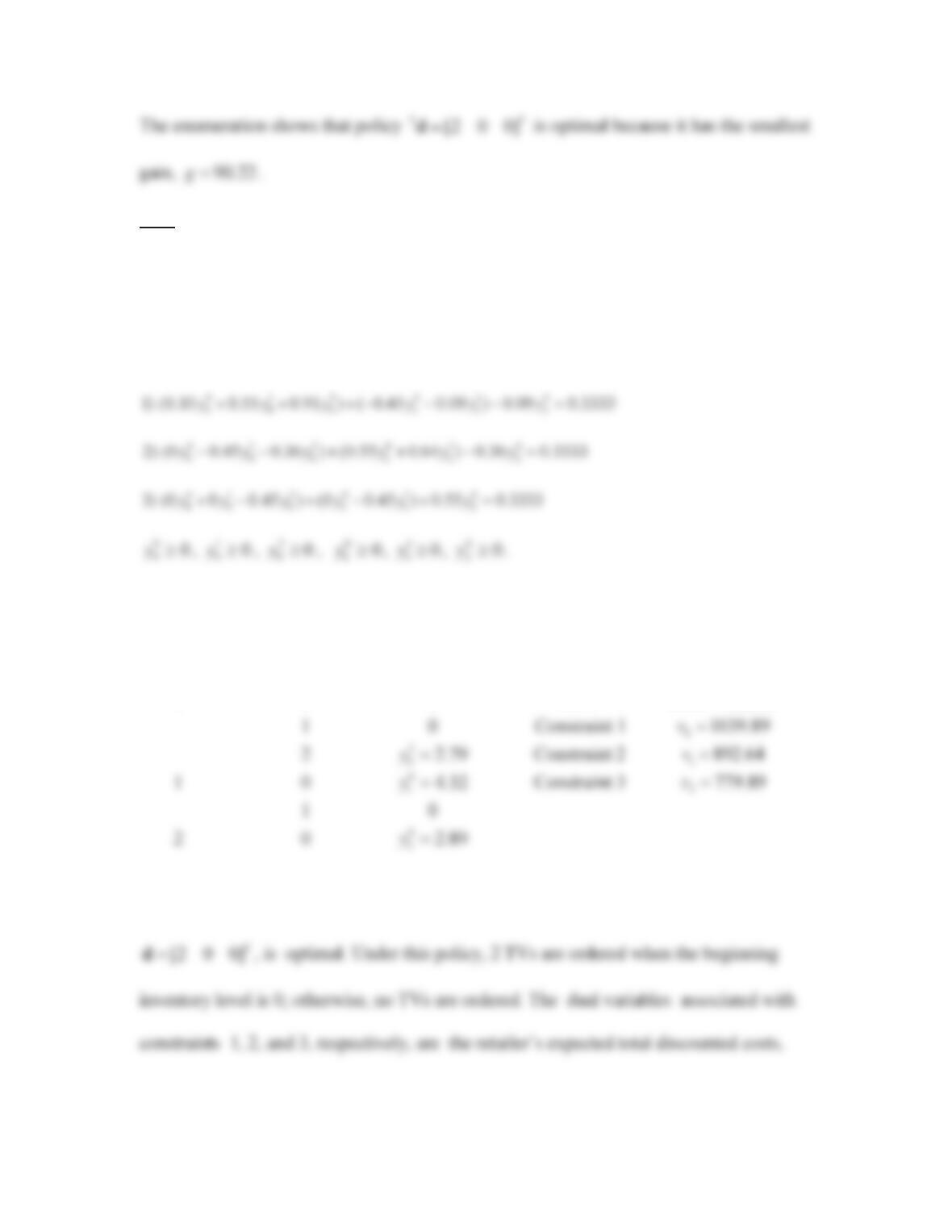
90.22, 260, 125.56, 0gvv v
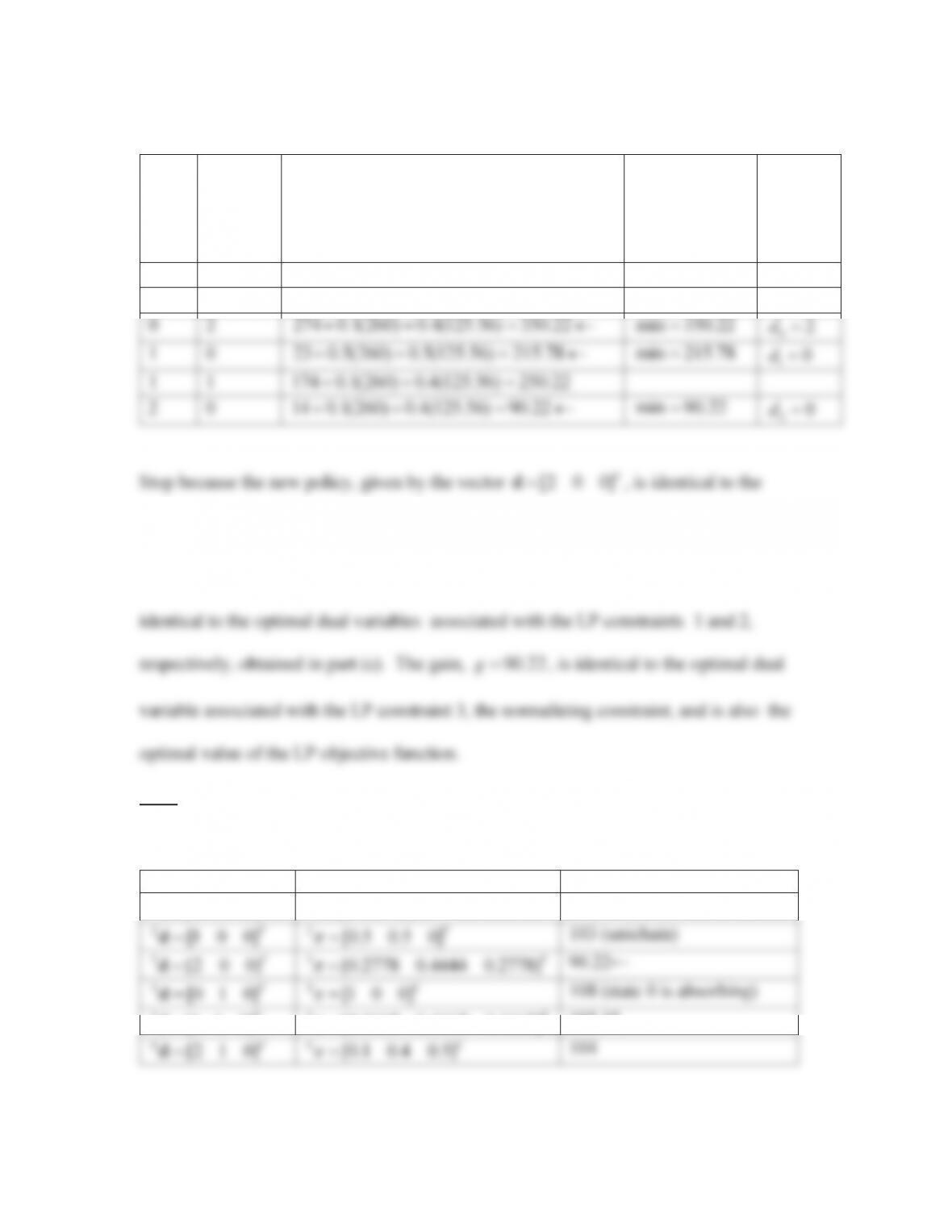
First policy improvement for inventory model
State Decision Test Quantity
State
i
Decision
Alterna-
tive
k
00 11 22
01 2
Test Quantity
(260) (125.56) (0)
kk k k
ii i i
kk k k
ii i i
qpvpvpv
qp p p
Minimum
Value of
Test
Quantity
Decision
kd
i
0
0
108 1(260) 0(125.56) 368
0
1
183 0.5(260) 0.5(125.56) 375.78
71
3[200]
T
5.3f) The linear programming formulation for the discounted MDP inventory model with
0.9
D
and
123
0.3333bbb
appears below.
Minimize
01 2 010
00 0 112
(108 183 274 ) (23 174 ) 14zyyy yyy
subject to
0ty
0ty
0ty
1
1
2
The solution of the discounted LP model is summarized below.
Objective function value, z 904.05
000
k
i
iky
Row Dual Variable
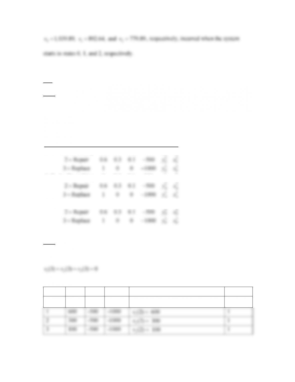
As in part (c) without discounting, a (1, 2) policy, given by the vector
T
72
1, 039.89, 892.64, and 779.89vv v
, respectively, incurred when the system
5.4)
5.4a) When an excellent machine is replaced and a poor machine is left alone, the MDP
model of machine maintenance is an absorbing multichain. The multichain MDP model
with LP variables added in the two right most columns is summarized below.
State Decision Transition Prob. Reward
,,,
11
11
E=1 1 Do nothing 0.1 0.7 0.2 600
A=2 1 Do nothing 0 0.4 0.6 300
P=3 1 Do no
kkk k kk
iE iA iP i i i
EE
AA
ikpppqyx
yx
yx
11
thing 0 0 1 100
PP
yx
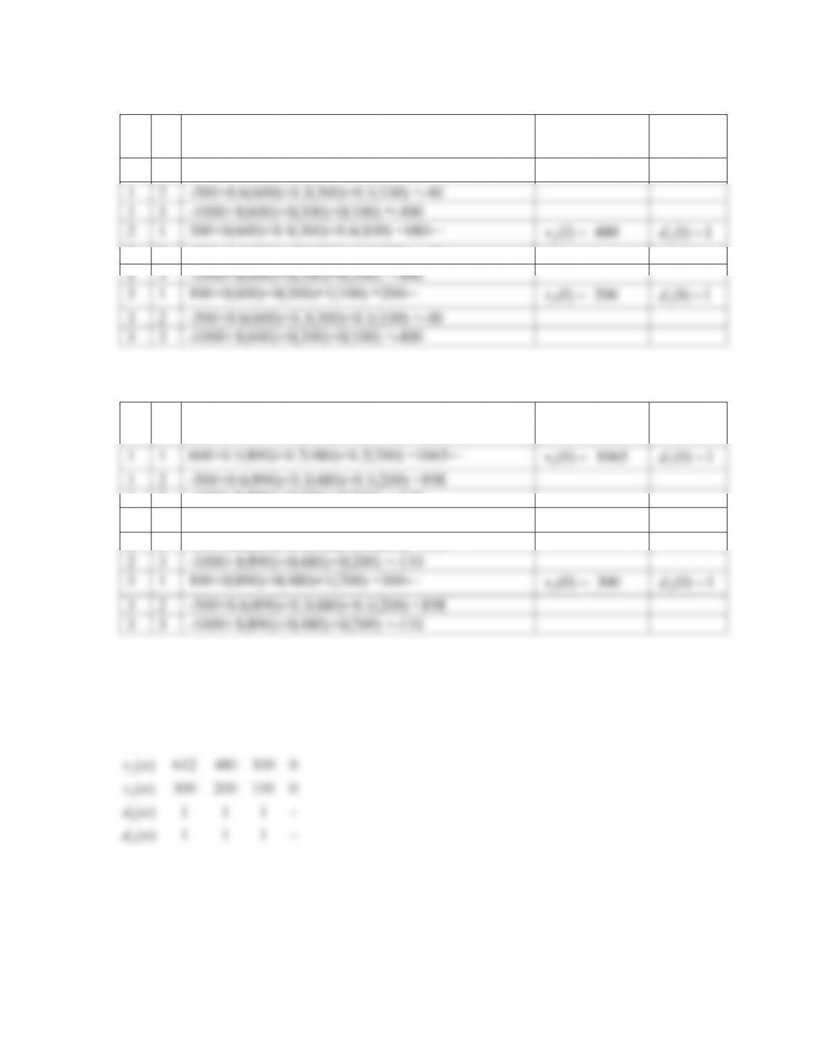
5.4b) To begin value iteration, assume zero expected total profits are received in every
state at the end of day 3.
123
(3) (3) (3) 0vvv
Value iteration for
2n
State
1
i
q
2
i
q
3
i
q
Expected Total Profit
Decision
i
1k
2k
3k
12 3
(2) max[ , , ]
iiii
k
vqqq
, for
1, 2, 3i
k
1
600
-500
-1000
1(2) 600v
1
2
300
-500
-1000
2
(2) 300v
1
3
100
-500
-1000
3(2) 100v
1
Value iteration for
1n
i
k
123
(600) (300) (100)
kk k k
ii i i
qp p p
(1)
i
v
(1)
i
dk
1
1
600+0.1(600)+0.7(300)+0.2(100) =890←
1(1) 890v
1
(1) 1d
1
2
-500+0.6(600)+0.3(300)+0.1(100) =-40
1
3
-1000+1(600)+0(300)+0(100) =-400
2
1
300+0(600)+0.4(300)+0.6(100) =480←
(1) 1d
2
2
-500+0.6(600)+0.3(300)+0.1(100) =-40
3
1
100+0(600)+0(300)+1(100) =200←
3
2
-500+0.6(600)+0.3(300)+0.1(100) =-40
1
1
600+0.1(890)+0.7(480)+0.2(200) =1065←
1
2
1
3
-1000+1(890)+0(480)+0(200) =-110
2
1
300+0(890)+0.4(480)+0.6(200) =612←
2
2
2
3
3
1
100+0(890)+0(480)+1(200) =300←
3
2
3
3
74
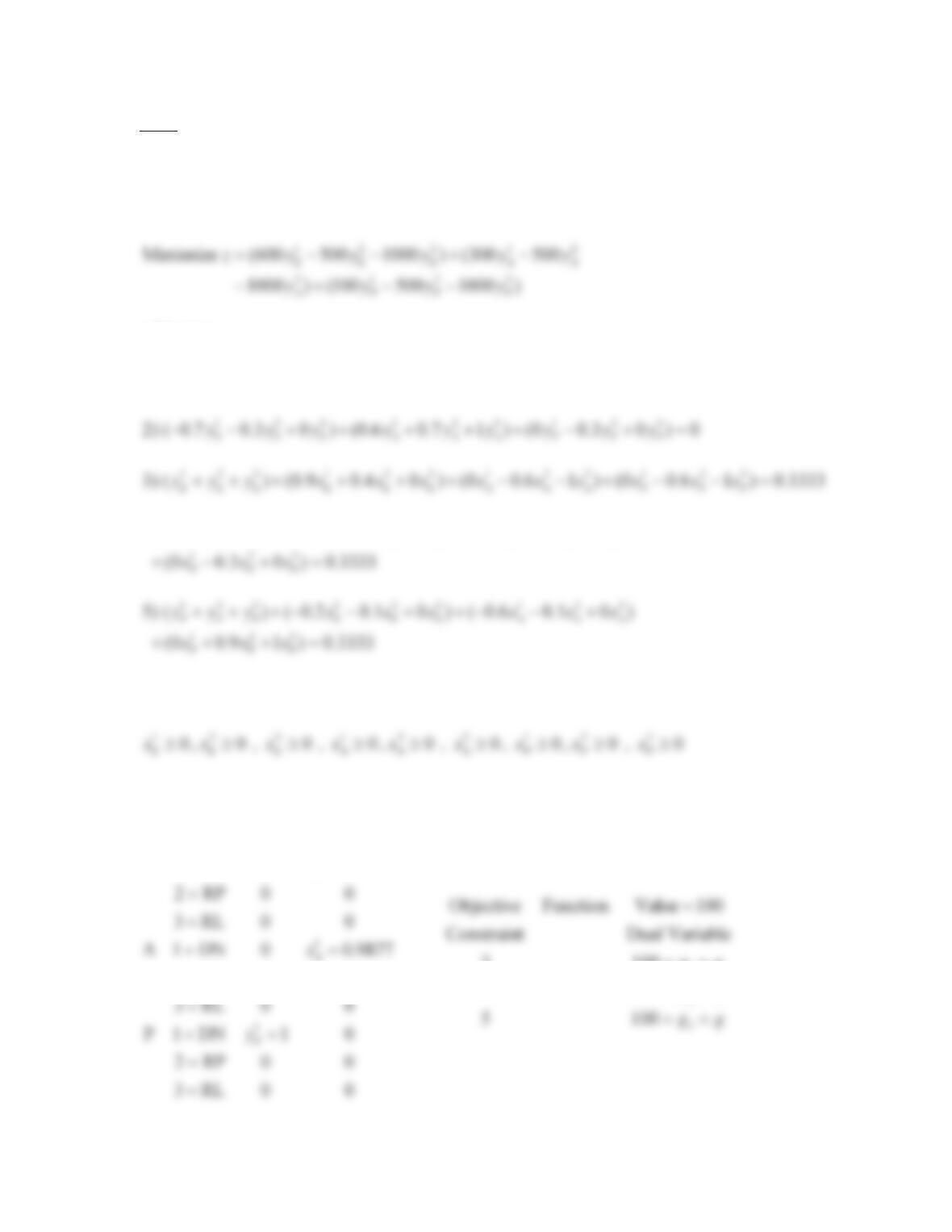
5.4c) After omitting a redundant constraint from the first set of constraints, the linear
programming formulation for the multichain MDP model of machine maintenance
appears below.
3123
1000 ) (100 500 1000 )
APPP
yyyy
subject to
123123123
1) (0.9 0.4 0 ) (0 0.6 1 ) (0 0.6 1 ) 0
EEEAAAPPP
yyyyyyyyy
EEE E E E A A A P P P
123 1 2 3 1 2 3
4) ( ) ( 0.7 0.3 0 ) (0.6 0.7 1 )
AAA E E E A A A
yyy x x x x x x
123
(0 0.9 1 ) 0.3333
PPP
xxx
10
E
yt
,
20
E
yt
,
30
E
yt
,
10
A
yt
,
20
A
yt
,
30
A
yt
,
10
P
yt
,
20
P
yt
,
30
P
yt
E
E
E
A
A
A
P
P
P
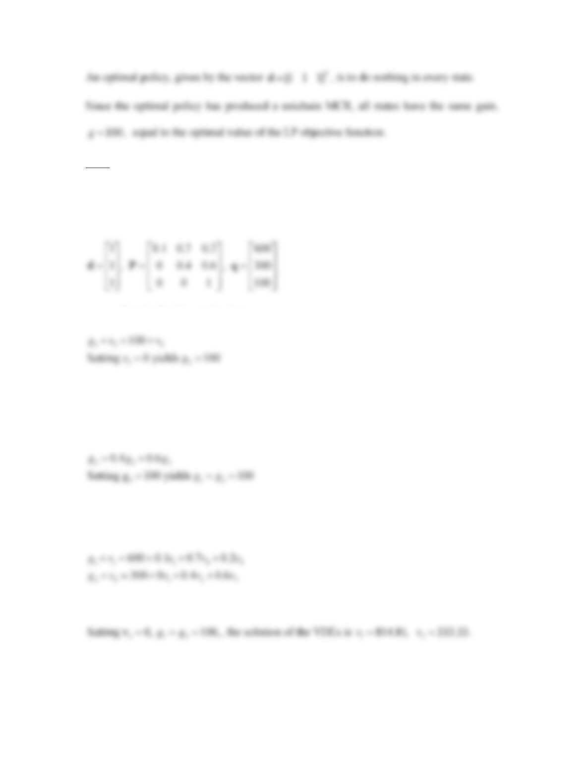
A solution of the multichain LP model is summarized below.
1
E 1 DN 0 0.3704
kk
ii
E
ik y x
x
75
T
5.4d) To begin policy iteration, arbitrarily choose the initial policy
[111]
T
d
. The
initial decision vector
d
, along with the associated transition probability matrix
P
and
the cost vector
q
, are shown below.
1 0 0 1 100
«» « » « »
«» « » « »
¬¼ ¬ ¼ ¬ ¼
Step 1 of policy evaluation:
33
100
Setting 0 yields 100
gv v
vg
Step 2 of policy evaluation:
The GSEs for the transient states are
1123
0.1 0.7 0.2
gggg
Step 3 of policy evaluation:
The VDEs for the transients states are
22 1 2 3
600 0.1 0.7 0.2
300 0 0.4 0.6
gv v v v
gv v v v
Step 4 of policy evaluation:
312
Setting v 0, 100,gg
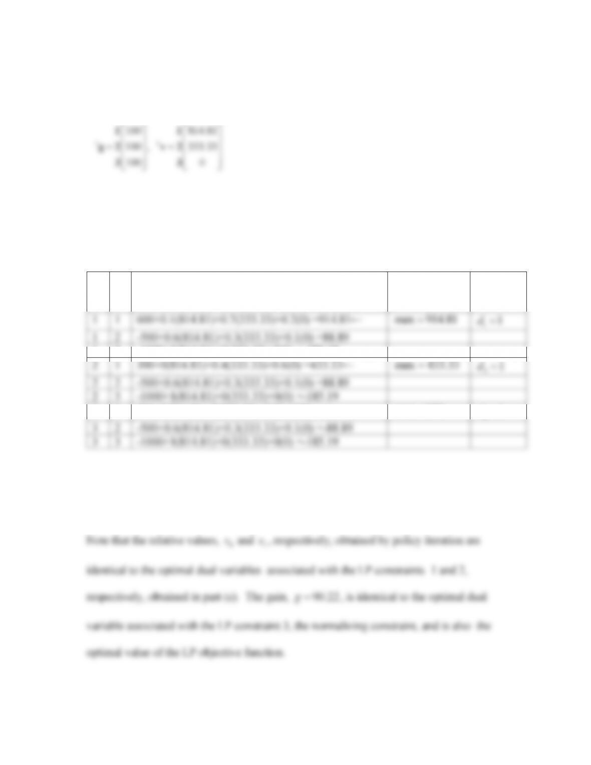
, the solution of the VDEs is
12
814.81, 333.33vv
.
76
The solutions for the gain vector and the vector of relative values for the initial policy are
summarized below.
100 814.81
100 , 333.33
100 0
ªº ª º
«» « »
«» « »
¬¼ ¬ ¼
11
g2 v2
33
Since the initial policy has produced a unichain MCR for which all states have the same
gain, the value test quantity will be calculated by the first policy improvement routine.
First policy improvement
State Decision Value Test Quantity
i
k
12 3
(814.81) (333.33) (0)
kk k k
ii i i
qp p p
Max Value of
Test
Quantity
Decision
kd
i
1
1
600+0.1(814.81)+0.7(333.33)+0.2(0) =914.81←
max 914.81
1
1d
1
2
-500+0.6(814.81)+0.3(333.33)+0.1(0) =88.89
1
3
-1000+1(814.81)+0(333.33)+0(0) =-185.19
2
1
300+0(814.81)+0.4(333.33)+0.6(0) =433.33←
max 433.33
2
1d
2
2
-500+0.6(814.81)+0.3(333.33)+0.1(0) =88.89
2
3
-1000+1(814.81)+0(333.33)+0(0) =-185.19
3
1
100+0(814.81)+0(333.33)+1(0) =100←
max 100
3
1d
3
2
-500+0.6(814.81)+0.3(333.33)+0.1(0) =-88.89
3
3
-1000+1(814.81)+0(333.33)+0(0) =-185.19
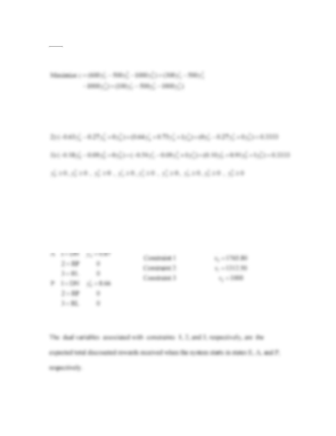
Stop because the new policy, given by the vector
[111]
T
d
, is identical to the
previous policy. Therefore, this policy is optimal.
77
5.4e) The linear programming formulation for the discounted MDP model of machine
maintenance with
0.9
D
appears below.
3123
1000 ) (100 500 1000 )
APPP
yyyy
subject to
123123123
1) (0.91 0.46 0.1 ) (0 0.54 0.9 ) (0 0.54 0.9 ) 0.3333
E EEA AAP PP
yyyyyyyyy
E
E
E
A
A
A
P
P
P
The solution of the discounted LP model is summarized below.
1
1
E1DN 0.36
2RP 0
3RL 0
k
i
E
ik y
y
Objective function value 1,345.84
Row Dual Variable
The optimal policy, given by the vector
[111]
T
d
, is to do nothing in every state.