Applied Statistics and Probability for Engineers, 7th edition 2017
5-18
Section 5-5
5.5.1 a) percentage of slabs classified as high with probability p1 = 0.05
b) X is the number of voids independently classified as high X 0
5.5.2 a) Probability for the kth landing page = pk = 0.25
Applied Statistics and Probability for Engineers, 7th edition 2017
5-19
5.5.3 Because
= 0 and X and Y are normally distributed, X and Y are independent. Therefore,
5.5.4 a)
Applied Statistics and Probability for Engineers, 7th edition 2017
5-20
b)
c)
5.5.5 Because
= 0 and X and Y are normally distributed, X and Y are independent. Therefore,
X = 0.1 mm,
X = 0.00031 mm,
Y = 0.23 mm,
Y = 0.00017 mm
5.5.6 a)
= cov(X,Y)/
x
y = 0.6, cov(X,Y) = 0.6(2)(5) = 6
Applied Statistics and Probability for Engineers, 7th edition 2017
5.5.7
−
−
−+
− − − −
==
2
2()
()
1
2 2 2
1
( , ) 2
Y
X
XY
y
x
XY
XY
f x y dxdy e dxdy
5.5.8 a) X1, X2 and X3 are binomial random variables when considered individually, that is, the marginal
probability distributions are binomial. Their joint distribution is multinomial.
= = =
1 1 2 2 3 3
( , , )
P X x X x X x
Section 5-6
5.6.1 a) E(3X + 2Y) = 3(2) + 2(6) = 18
5.6.3 a) X N(0.1, 0.00031) and Y N(0.23, 0.00017) Let T denote the total thickness.
5.6.4 a) X: time of wheel throwing. X ~ N(40,4)
5.6.5 X = time of ACL reconstruction surgery for high-volume hospitals.
5.6.6 a) Let
X
denote the average fill-volume of 100 cans
==
2
0.5 100 0.05
X
5.6.7 X ~ N(160, 900)
5.6.8 D = A − B − C
5-23
5.6.9
12
( ) (2 2 )
V Y V X X
=+
5.6.10 Let Y be the rate of return for the entire investment after one year,
5.6.11 Let Xi be the demand in month i.
a)
1 2 12
…
Z X X X
= + + +
Applied Statistics and Probability for Engineers, 7th edition 2017
5-24
Section 5-7
5.7.1
1
() 4
Y
fy=
at y = 3, 5, 7, 9
−
−
1
2
1
y
e
5.7.4 a) Now,
2
0
bv
av e dv
−
must equal one. Let u = bv, then
2
2
3
00
1uu
udu a
a e u e du
b
bb
−−
==
. From the
5.7.5 If y = ex, then x = ln y for 1 ≤ x ≤ 2 and e1 ≤ y ≤ e2. Thus,
11
( ) (ln )
YX
f y f y yy
==
for 1 ≤ ln y ≤ 2.
5.7.6
ln
W
Ye
WY
=
=
5.7.7
( )
= + + − 0.5
22
1 2 1 2 1 2
(cos cos )rrrrr
Applied Statistics and Probability for Engineers, 7th edition 2017
5-25
Then, f(r) = f(
2)|J|, where
5.7.8 Here, X is lognormal with
= 5.2933, and
2 = 0.00995
Y = X4
Section 5-8
5.8.1 a)
−−
+
= = =
−
= = = = = −
11
( 1)
1 0 0
1 1 (1 )
( ) ( ) (1 )
t t tm
m m m
tX tx t x tx
Xt
x x x
e e e
M t E e e e e
m m m me
Applied Statistics and Probability for Engineers, 7th edition 2017
5-26
5.8.3 a)
−
==
= = − = −
−
1
11
( ) ( ) (1 ) ( (1 ))
1
tX tx x t x
X
xx
p
M t E e e p p e p
p
b)
( ) ( )
( )
=
=
− − − − −
= = = = −−
12
0
0
1 (1 ) (1 )
()
( ) ‘
1 (1 )
t t t t
X
t
t
t
pe p e pe p e
dM t
EX dt pe
5.8.5 a)
−−
==
= = =
2 ( 2)
00
( ) ( ) (4 ) 4
tX tx x t x
X
xx
M t E e e xe dx xe dx
Applied Statistics and Probability for Engineers, 7th edition 2017
5-27
5.8.6
a)
=
=
−
= = = = − =
− − − −
1 1 1
( ) ( ) ()
x
tx t t t t
tX tx
X
x
e e e e e
M t E e e dx t t t t
( ) ( )
→
− − − + −
=−
2 2 2
23
0
2 2 2
‘ lim ()
t t t t t t
t
t e e t e e e e
t
5.8.7 a)
−−
= = =
()
( ) ( )
tX tx x t x
X
M t E e e e dx e dx
Applied Statistics and Probability for Engineers, 7th edition 2017
5-28
5.8.8 a)
( )
−− − −
= = =
11 ( )
00
( ) ( ) ( ) ( )
r
r
tX tx x r t x
X
M t E e e x e dx x e dx
rr
−−
1 ( )
0
r t x
x e dx
is finite only if t < λ. Besides, we need to use integration by substitution by
a)
( ) ( )
−− − −
==
==
= = = = − = − = − =
1
100
00
()
( ) ‘ 1
rrr
rr
X
tt
tt
dM t t r
E X t r t
dt
5.8.9 a)
= = =
− − − −
12
( ) ( ). ( )… ( ) …
r
r
Y X X X
M t M t M t M t t t t t
5.8.10 a)
= = + +
12
2 2 2 2
12
12
( ) ( ) ( ) exp exp
22
Y X X
tt
M t M t M t t t
Applied Statistics and Probability for Engineers, 7th edition 2017
5-29
Supplemental Exercises
5.S11 The sum of
=
( , ) 1
xy
f x y
,
+ + + + =
1 1 1 1 1 1
4 8 8 4 4
and fXY(x,y) ≥ 0
5.S12 a)
= = = = =
2 4 14
20!
( 2, 4, 14) 0.10 0.20 0.70 0.0631
P X Y Z
Applied Statistics and Probability for Engineers, 7th edition 2017
5-30
5.S13
= = =
3 2 3 23
23
22
00
0 0 0
2 18
23
yx
cx ydydx cx dx c c
. Therefore, c = 1/18.
5.S14 The region x2 + y2 ≤ 1 and 0 < z < 4 is a cylinder of radius 1 (and base area π) and height 4.
Therefore, the volume of the cylinder is 4π and
=1
( , , ) 4
XY Z
f x y z
for x2 + y2 ≤ 1 and 0 < z < 4.
Applied Statistics and Probability for Engineers, 7th edition 2017
5-31
5.S15 Let X, Y, and Z denote the number of problems that result in functional, minor, and no defects,
respectively.
c) E(Z) = 10(0.3) = 3
5.S16 a) Let
X
denote the mean weight of the 25 bricks in the sample. Then,
=( ) 3E X
and
5.S17 Let
X
denote the average time to locate 10 parts. Then,
=4( 5)E X
and
=30
10
X
5.S18 a) Let X denote the weight of a piece of candy and X N(0.1, 0.01). Each package has
Applied Statistics and Probability for Engineers, 7th edition 2017
5-32
5.S19
5.S20 a) Let Y denote the weight of an assembly. Then, E(Y) = 4 + 5.5 + 10 + 8 = 27.5 and V(Y) = 0.42 +
5.S21 Let T denote the total thickness. Then, T = X1 + X2 and
5.S22 Let X and Y denote the percentage returns for security one and two, respectively.
If half of the total dollars is invested in each, then 1/2X + 1/2Y is the percentage return.
5.S23 a) Let X, Y, and Z denote the risk of new competitors as no risk, moderate risk,
Applied Statistics and Probability for Engineers, 7th edition 2017
5-33
5.S24
Y X X Y
==
Then
5.S25
2
I
P I PR
R
==
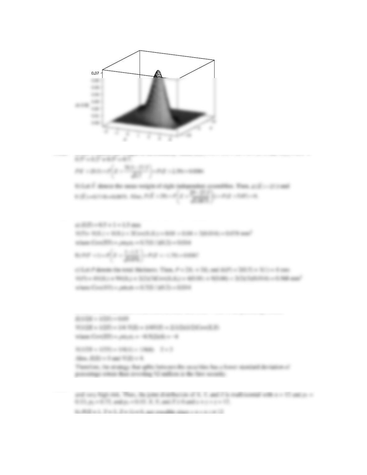
5.S26 Because the covariance is zero, one may consider a cross section of the beam, say along the
x axis. The distribution along the x axis is