Preliminaries: Lipschitz Condition (3)
Note that, in the previous example, the Lipschitz constant K was
given by the point in R where
This is true more generally:
Existence and Uniqueness Theorem
),( ytf
t
y
0
y
0
t
b
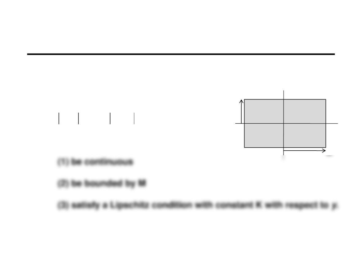
Let the function be defined on
the rectangle
R:
R
att − 0
byy − 0
and in R let :
),( ytf
Existence and Uniqueness Theorem (2)
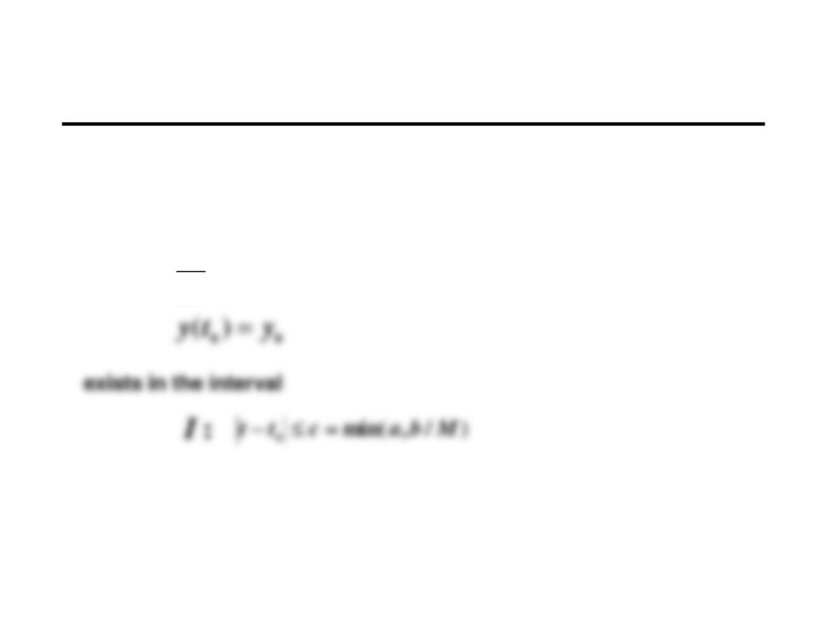
Then a unique solution to the first order ODE
),(
ytf
dt
dy
=
Successive Approximations and Convergence
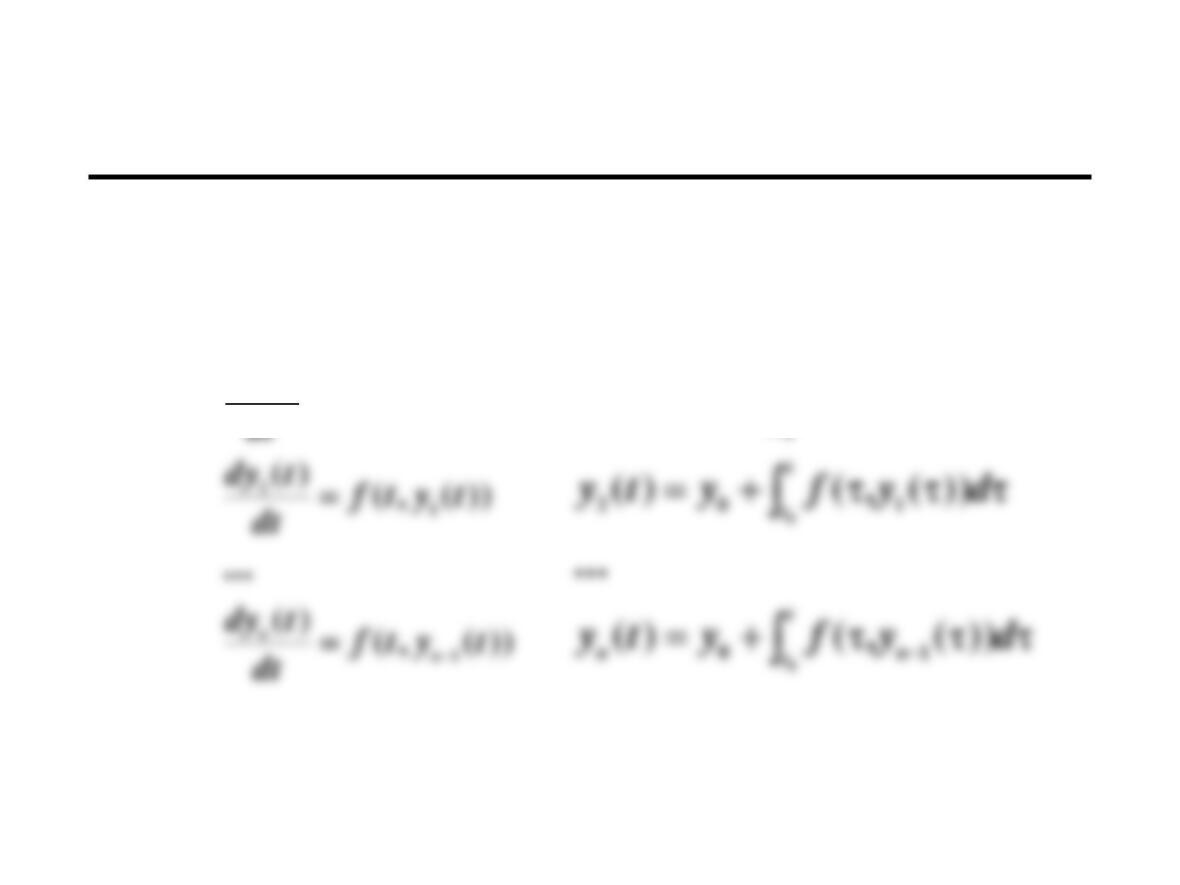
The sequence of approximations given by
converges to the solution of the ODE.
)(tyn
))(,(
)(
)(
0
0
tytf
tdy
yty
=
=
+=
dttytfyty
t
t
))(,()(
001
Successive Approximations and
Convergence (2)
Proof:
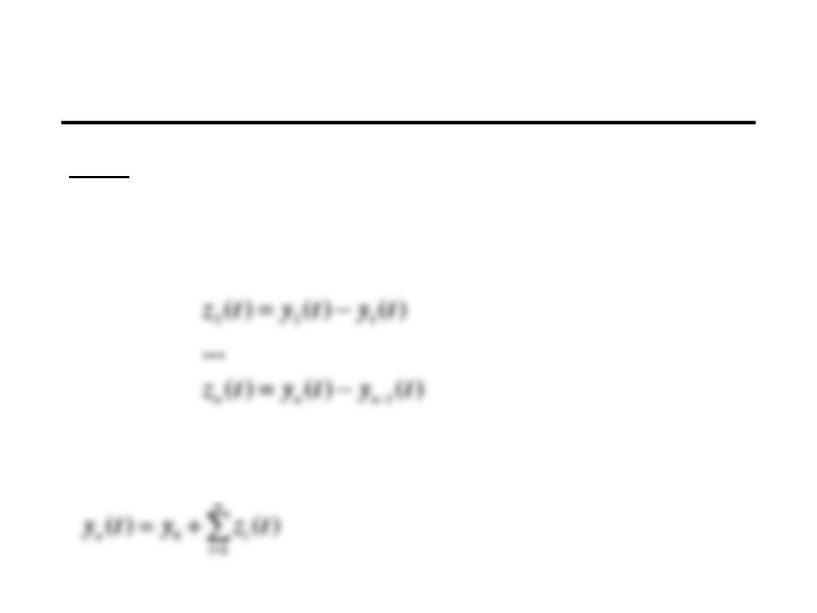
Consider the sequence of functions
Note that
)()(
011
ytytz
−=
−
−++−+−+=
nnn
tytytytytytyyty
112010
))()((…))()(())()(()(
Successive Approximations and
Convergence (3)
We must show that the series converges.
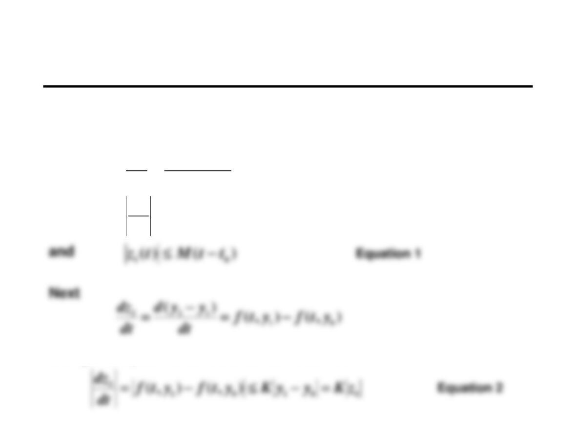
Now
Hence
Using the Lipschitz condition, this becomes
=
n
i
itz
1
)(
),(
)(
1
0
011
M
dt
dz
ytf
dt
yyd
dt
dz
=
−
=
Successive Approximations and
Convergence (4)
Using Equation 1 in Equation 2 and integrating, we obtain
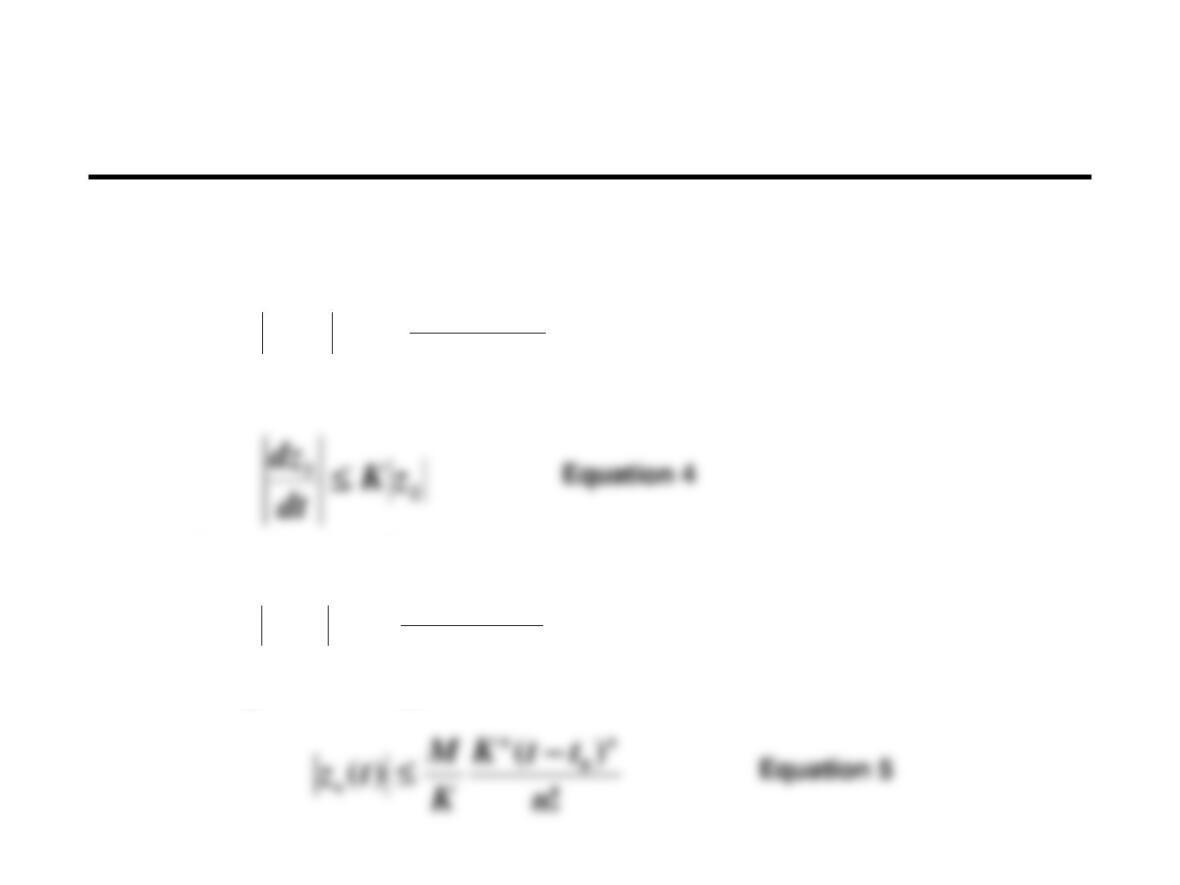
In the same way,
Using Equation 3 in Equation 4 and integrating, we obtain
Proceeding in this way, we find that
2
)(
)(
2
0
2
ttK
Mtz −
Equation 3
23
)(
)(
3
0
2
3
−
ttK
Mtz

Successive Approximations and
Convergence (5)
From Equation 5, each element of the series is smaller
term by term than the nth element of a convergent series, namely that
=
n
i
itz
1
)(
Some Solutions Are Local
Example 1:
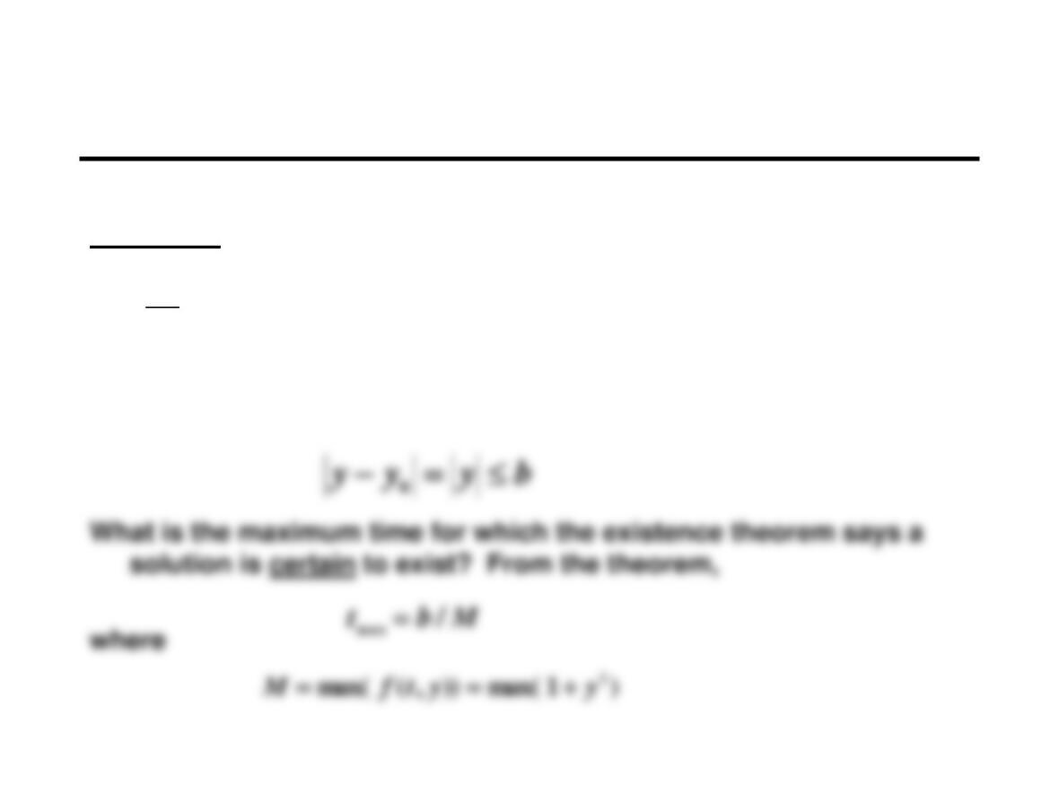
The function satisfies a Lipschitz condition only if
we limit the magnitude of . Let
2
1y
dt
dy +=
0)0( =y
2
1),( yytf +=
y
Some Solutions Are Local (2)
Since
Then
22 11 by
by
++

Some Solutions Are Local (3)
The solution of
2
1y
dt
dy +=
0)0( =y
Some Solutions Are Local (4)
Example 2: Consider the three ODEs:
2
1y
dt
dy +=
0)0( =y
(1)
Some Solutions Are Local (5)
The solution of the second ODE is
It goes to infinity as
t
t
ty −
=1
)(

Key Aspects of
Existence and Uniqueness Theorems
Existence of a solution is proved by demonstrating a reliable process
(successive approximations) for computing one

Homework Assignment 5
Read: Chapter 4, Sections 4.1 through 4.4