Applied Statistics and Probability for Engineers, 7th edition 2017
CHAPTER 4
Section 4.1
= = = − − =
00
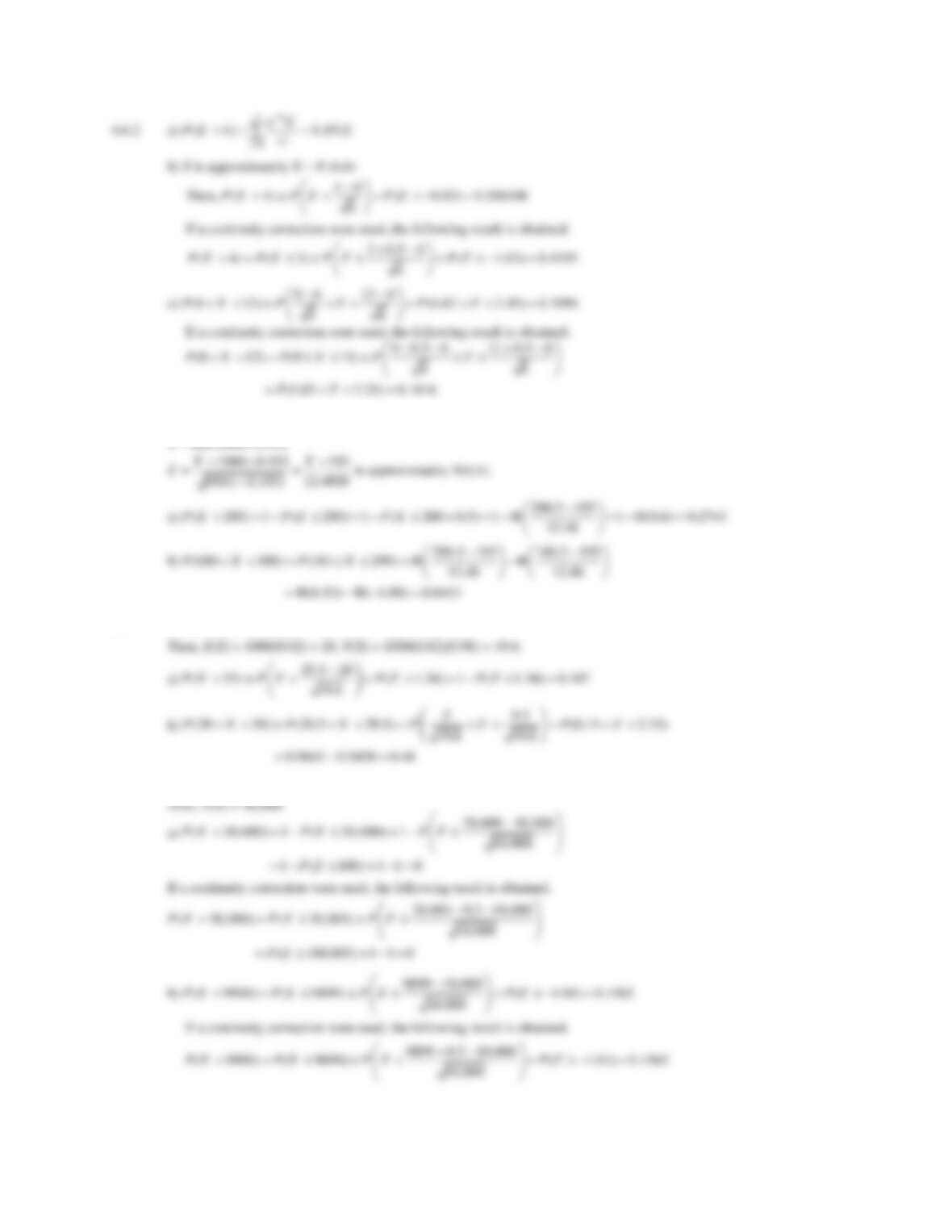
( 0) 0.5cos (0.5sin ) 0 ( 0.5) 0.5P X xdx x
Applied Statistics and Probability for Engineers, 7th edition 2017
4.1.4 a)
−
= = = =
4
42 2 2
43
( 4) 0.4375
xx
P X dx
, because fX (x) = 0 for x < 3.
4.1.5 a) P(0 < X) = 0.5, by symmetry.
4.1.6 a)
= = =
50.25 50.25
50
50
( 50) 2.0 2 0.5P X dx x
4.1.7 a) P(X < 2.25 or X > 2.75) = P(X < 2.25) + P(X > 2.75) because the two events are mutually exclusive. Then,
4.1.8 a) P(X < 90) = 0 because the pdf is not defined in the range (−∞, 90).
Applied Statistics and Probability for Engineers, 7th edition 2017
d) Find a such that P(X > a) = 0.1
4.1.9 a)
= − = − − =
0.5 0.5
0
( 0.5) 0.5exp( 0.5 ) exp( 0.5 ) 0.221P X x dx x
4.1.10 a)
= − = −
40 40
2
30
( 40) (0.0025 0.075) (0.00125 0.075 )
P X x dx x x
Section 4.2
4.2.1 a) P(X < 2.8) = P(X 2.8) because X is a continuous random variable.
Applied Statistics and Probability for Engineers, 7th edition 2017
4.2.4 Now,
=3
2
()fx x
for x > 1 and
4.2.7 Now, f(x) = 2 for 2.3 < x < 2.8 and
= = −
( ) 2 2 4.6
x
F x dy x
Applied Statistics and Probability for Engineers, 7th edition 2017
For 50 ≤ x < 70,
0, 0
x
x
4.2.12 For 100 ≤ x < 500,
Section 4.3
4.3.1
−−
= = =
1
14
3
11
( ) 1.5 1.5 0
4
x
E X x dx
Applied Statistics and Probability for Engineers, 7th edition 2017
4.3.2
= = =
4
43
2
00
( ) 0.125 0.125 2.6667
3
x
E X x dx
4.3.3
−
=
1
() x
E X xe dx
. Use integration by parts to obtain
4.3.4
= − = −
50
50 32
( ) (0.0025 0.075) 0.0025 0.075
32
xx
E X x x dx
4.3.5 Probability distribution from exercise 4.1.8 used.
Here, a = 5.56E − 6, b = −5.56E − 4, c = −4.44E − 6, d = 4.44E − 3
4.3.6 a)
= = =
1210 1210
2
1200
1200
( ) 0.1 0.05 1205
E X x dx x
Applied Statistics and Probability for Engineers, 7th edition 2017
4.3.7 a)
= = =
120 120
2100
100
600
( ) 600 ln 109.39E X x dx x
x
Section 4.4
4.4.1 a) E(X) = (−1+1)/2 = 0
4.4.2 a) The distribution of X is f(x) = 10 for 0.95 < x < 1.05. Now,
= −
0, 0.95
( ) 10 9.5, 0.95 1.05
X
x
F x x x
4.4.3 a) The distribution of X is f(x) = 100 for 0.2050 < x < 0.2150. Therefore,
0, 0.2050
x
4.4.4 Let X denote the changed weight.
4.4.6 a) E(X) = (380 + 374)/2 = 377
4.4.7 a) Let X be the arrival time (in minutes) after 9:00 A.M.
4.4.8 Let X denote the kinetic energy of electron beams.
a)
+
= = =
37
( ) 5
EX
12
Section 4.5
4.5.1 a) P(Z < 1.32) = 0.90658
b) P(Z < 3.0) = 0.99865
4.5.2 a) Because of the symmetry of the normal distribution, the area in each tail of the distribution must equal 0.025.
Therefore, the value in Table III that corresponds to 0.975 is 1.96. Thus, z = 1.96.
4.5.3 a) P(X < 13) = P(Z < (13−10)/2) = P(Z < 1.5) = 0.93319
4.5.4 a)
−
==
1
() 00.5
P X x x
PZ
. Therefore,
−=
10 0
x
and x = 10.
4.5.5 a) 1 –
(2) = 0.0228
4.5.6 a) Let X denote the time.
Applied Statistics and Probability for Engineers, 7th edition 2017
−
0.5 0.4
4.5.8 Let X denote the cholesterol level.
X ~ N(159.2,
2
)
4.5.9 Let X denote the height.
X ~ N(1.41, 0.012)
4.5.10 Let X denote the height.
X ~ N(64, 22)
Applied Statistics and Probability for Engineers, 7th edition 2017
4.5.11 a)
−
= = − =( 5000) (
5000 7000 3
600 .33) 0.00043PZP X P Z
4.5.12 Let X denote the demand for water daily.
X ~ N(310, 452)
4.5.13 a)
−
=
= =
13 12
( 13) ( 2)
4.5.14 a)
−
=
= =
=
0.0026 0.002
(0 ( 1.5) 1.0026) 0.0 ( 1.5) 0.06 1
468
00
PPZX P Z PZ –
4.5.15 From the shape of the normal curve, the probability is maximized for an interval symmetric about the mean. Therefore a
Applied Statistics and Probability for Engineers, 7th edition 2017
4.5.16 a)
−
= =
=
( 10) ( 1.8621) 0.0
10 4 31
.6
2. 3
9
PZP X P Z
4.5.17 a)
−
= = =( 100) (
100 1.964) 0.0
50 2
.9
24
58PZP X P Z
4.5.18 Let X denote the value of the signal.
4.5.20 Let X1 and X2 denote the right ventricle ejection fraction for PH subjects and control subjects, respectively.
Section 4.6
Applied Statistics and Probability for Engineers, 7th edition 2017
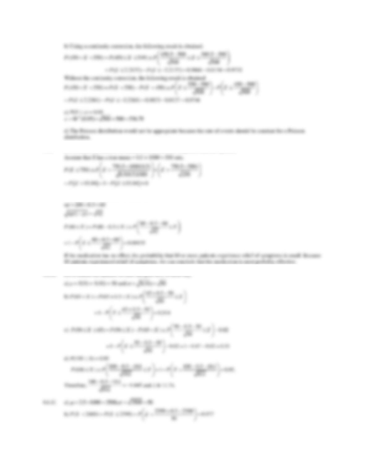
4.6.3 Let X denote the number of people with a disability in the sample.
4.6.4 Let X denote the number of defective chips in the lot.
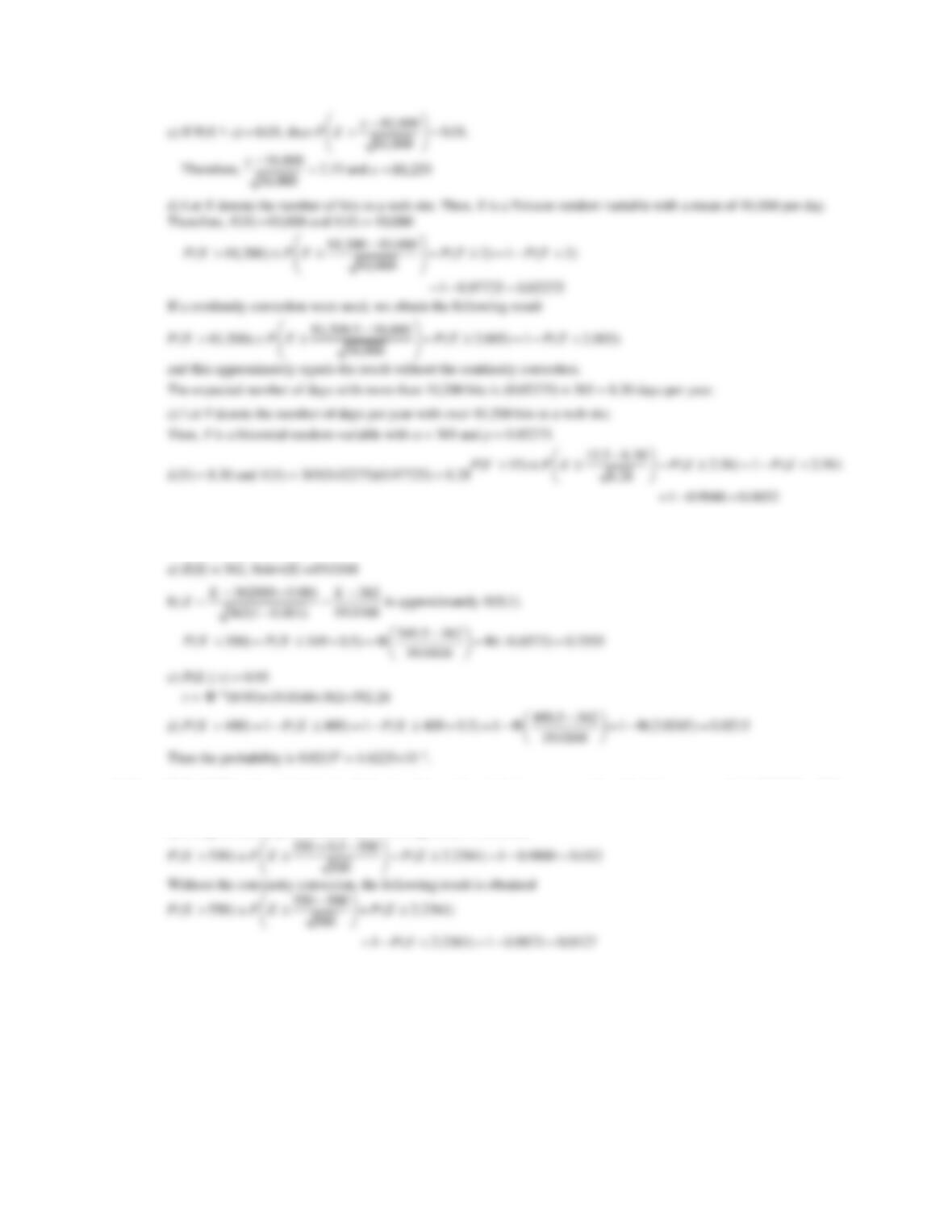
4.6.5 Let X denote the number of hits to a web site. Then, X is a Poisson random variable with a mean of 10,000 hits per day.
Applied Statistics and Probability for Engineers, 7th edition 2017
4.6.6 Let X denote the number of accounts in error in a month.
X ~ Bin(362,000, 0.001)
4.6.7 With 10,500 asthma incidents in children in a 21-month period, then mean number of incidents per month is 10500/21 = 500.
Let X denote a Poisson random variable with a mean of 500 per month. Also, E(X) =
= 500 = V(X).
a) Using a continuity correction, the following result is obtained.
Applied Statistics and Probability for Engineers, 7th edition 2017
4.6.8 Let X denote the number of random sets that is more dispersed than the opteron.
4.6.9 Approximate with a normal distribution.
4.6.10 Let X denote the number of cabs that pass in a 10-hour day.
Applied Statistics and Probability for Engineers, 7th edition 2017
Section 4.7
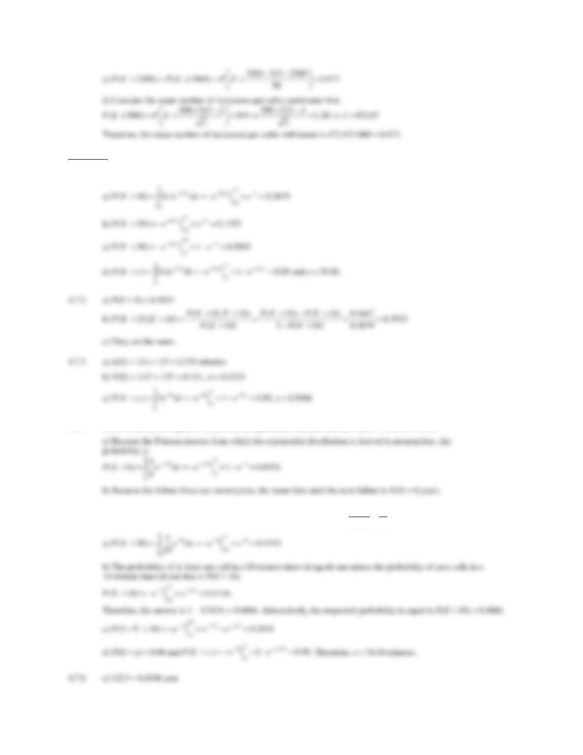
4.7.1 If E(X) = 10, then
= 0.1.
4.7.4 Let X be the life of regulator. Then, X is an exponential random variable with
==1/ ( ) 1/ 6EX
.
4.7.5 Let X denote the time until the first call. Then, X is exponential and
==
11
( ) 15EX
calls/minute.
Applied Statistics and Probability for Engineers, 7th edition 2017
4.7.7 Let X denote the time until the arrival of a taxi. Then, X is an exponential random variable with
= 1/E(X) = 0.1
arrivals/minute.
4.7.8 Let X denote the distance between major cracks. Then, X is an exponential random variable with
= 1/E(X) =
0.2 cracks/mile.
4.7.9 Let X denote the number of insect fragments per gram. Then
= 14.4/225
4.7.10 Let Y denote the number of arrivals in 1 hour. If the time between arrivals is exponential, then the count of arrivals is a
Poisson random variable and
= 1 arrival per hour.
Applied Statistics and Probability for Engineers, 7th edition 2017
4.7.11 Let X denote the number of calls in 30 minutes. Because the time between calls is an exponential random variable, X is a
Poisson random variable with
==1/ ( ) 0.1EX
calls per minute. Therefore, E(X) = 3 calls per 30 minutes.
4.7.12
−
=
( ) .
x
E X x e dx
Use integration by parts with u = x and dv =
e−
x.