CHAPTER 3 REDUCIBLE MARKOV CHAINS
3.1) )
3.1a)
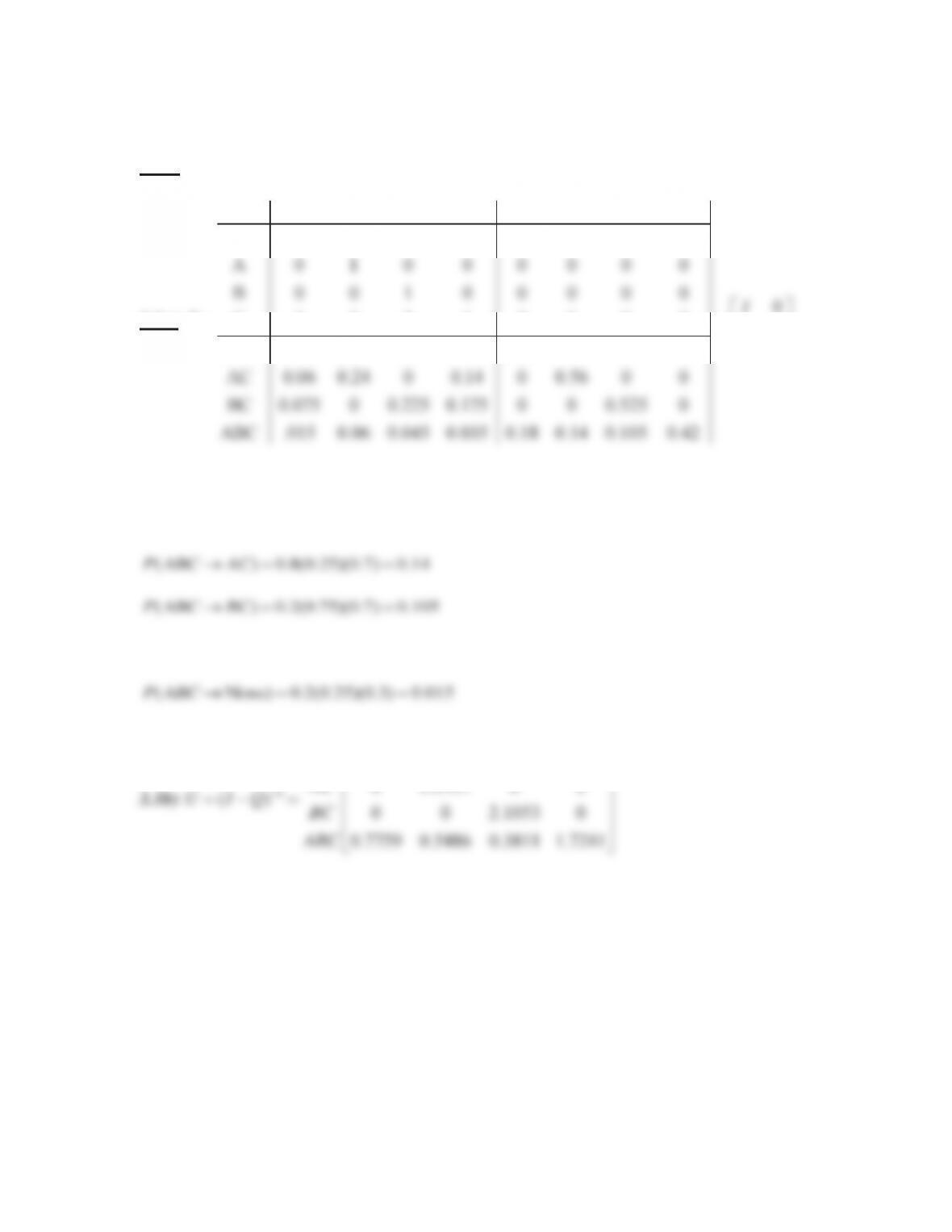
States None A B C AB AC BC ABC
None 1 0 0 0 0 0 0 0
C 000 1000 0
AB 0.05 0.20 0.15 0 0.60 0 0 0
AC 0.06 0.24 0 0.14 0 0.56 0 0
BC 0.075 0 0.225 0.175 0 0 0.525 0
ABC .015 0.06 0.045 0.035 0.18 0.14 0.105 0.42
I
PDQ
ªº
«»
¬¼
Calculations of the transition probabilities out of state ABC are shown below.
035.0)7.0)(25.0(2.0)( oCABCP
42.0)7.0)(75.0(8.0)( o ABCABCP
22
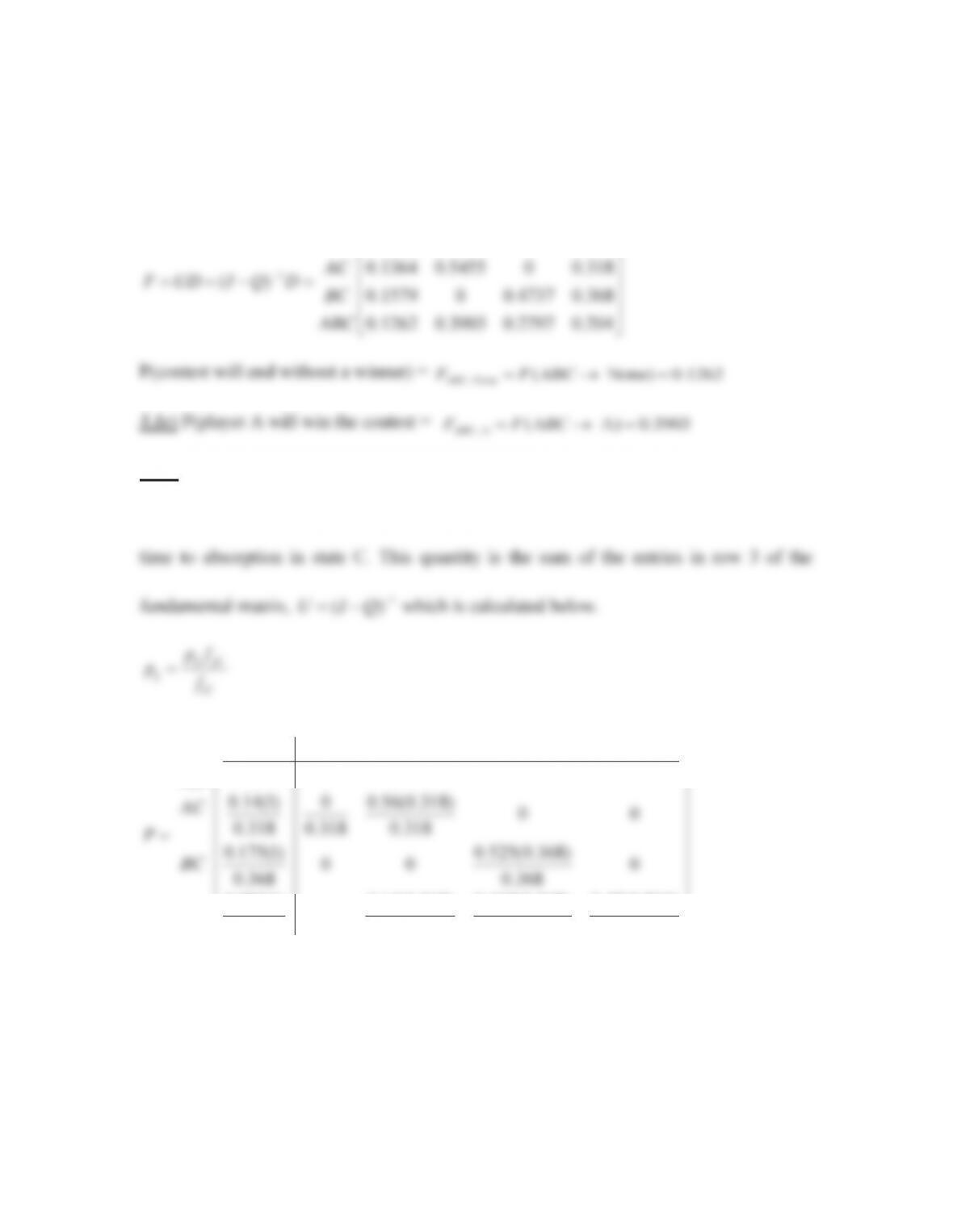
0.125 0.5 0.375 0
NONE A B C
AB
ªº
, A
ABC
3.1d) If players B and C are the remaining contestants,
the expected number of rounds needed before C wins equals 2.1053, the conditional mean
ij
iC
678
10 0 0 0
00 0 0 0
0.035(1) 0.14(0.318) 0.105(0.368) 0.42(0.204)
0
0.204 0.204 0.204 0.204
C
C
ABC
ªº
«»
«»
«»
«»
¬¼
23
100 0 0
000 0 0 0
C
AB I
ªº
«»
«»
ªº
¬¼
3.2)
3.2a)
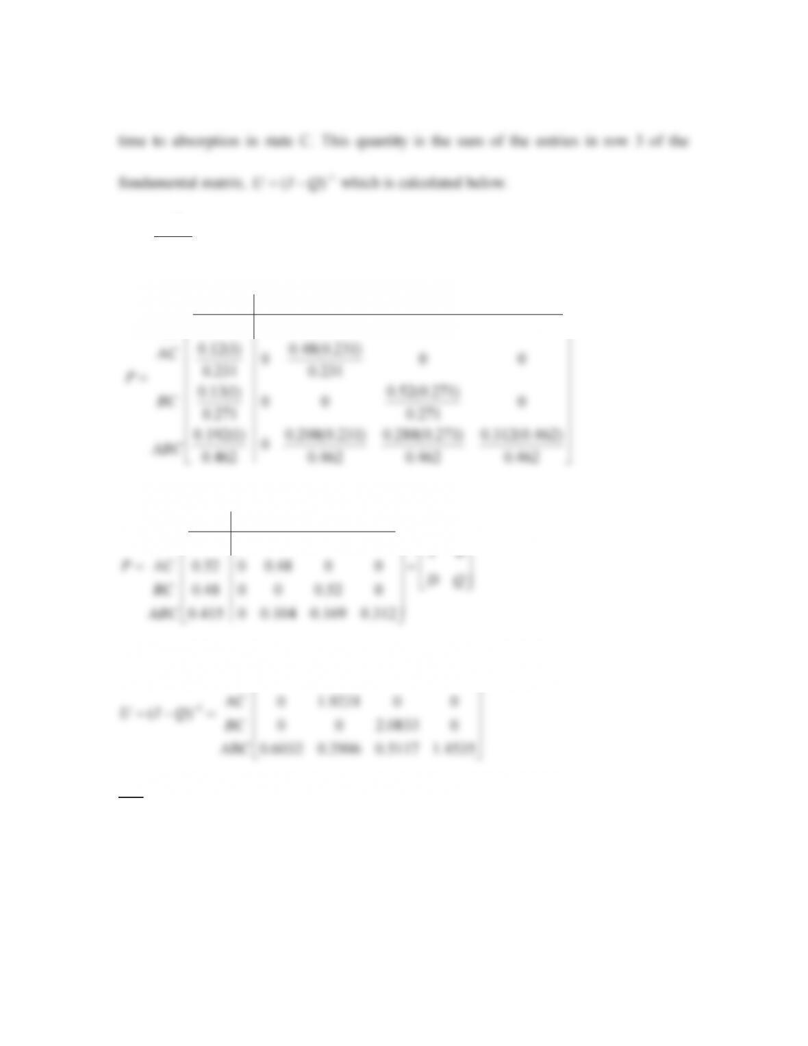
States None A B C AB AC BC ABC
None100000 0 0
C00010000
I
PDQ
ªº
«»
Calculations of the transition probabilities out of state AC are shown below.
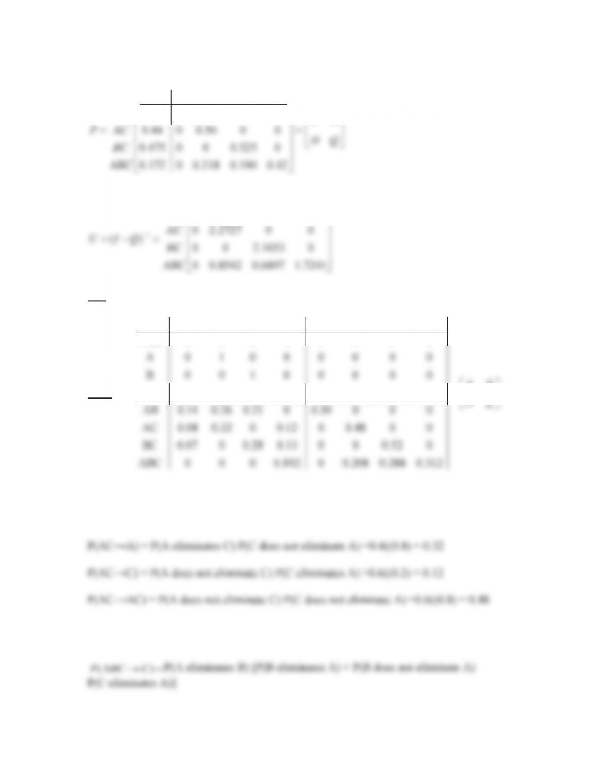
P(AC→None) = P(A eliminates C) P(C eliminates A) =0.4((0.2) = 0.08
Calculations of the transition probabilities out of state ABC are shown below.
24
o )( ACABCP
P(A eliminates B) P(B does not eliminate A) P(C does not eliminate A)]
o )( BCABCP
P(A does not eliminate B) [P(B eliminates A) + P(B does not eliminate
3.2b)
1.6393 0 0 0
AB
ªº
¬¼
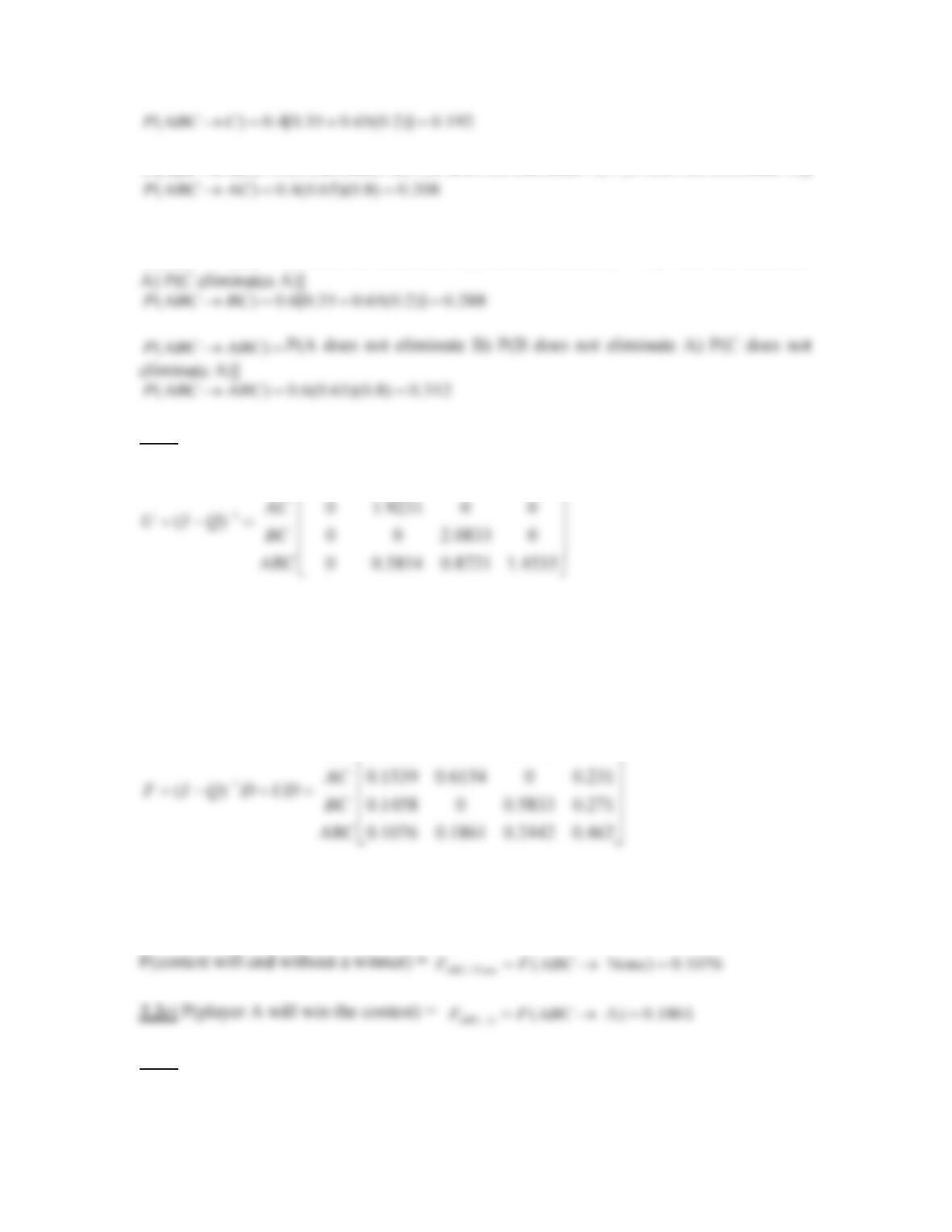
0.2295 0.4262 0.3443 0
NONE A B C
AB
ªº
¬¼
, A ( A) 0.1861
ABC
3.2d) If players B and C are the remaining contestants,
25
the expected number of rounds needed before C wins equals 2.0833, the conditional mean
ij jC
ij
iC
pf
pf
678
10 0 0 0
00 0 0 0
C
C
AB
ªº
«»
«»
10000
00000 0
C
AB I
ªº
«»
¬¼
3.3)
26
3.3a)
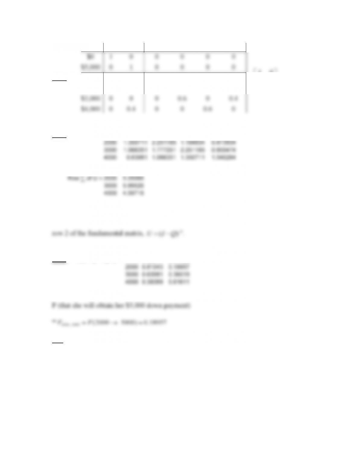
State $0 $5,000 $1,000 $2,000 $3,000 $4,000
$1,000 0.6 0 0 0.4 0 0
$2,000 0 0 0.6 0 0.4 0
I
PDQ
ªº
«»
¬¼
1000
2000
3000
4000
3.3b) U = (I – Q)-1 =1000
1.540284
0.900474
0.473934
0.189573
2000
1.350711
2.251185
1.184834
0.473934
3000
1.066351
1.777251
2.251185
0.900474
4000
0.63981
1.066351
1.350711
1.540284
1000
3.10427
Row ∑ of U = 2000
5.26066
3000
5.99526
4000
4.59716
The expected number of bets that she will make equals 5.26066, the sum of the entries in
1
0
5000
3.3c) F = UD = (I – Q)
-1
D = 1000
0.92417
0.07583
2000
0.81043
0.18957
3000
0.63981
0.36019
4000
0.38389
0.61611
2000, 5000
3.4)
27
3.4a)
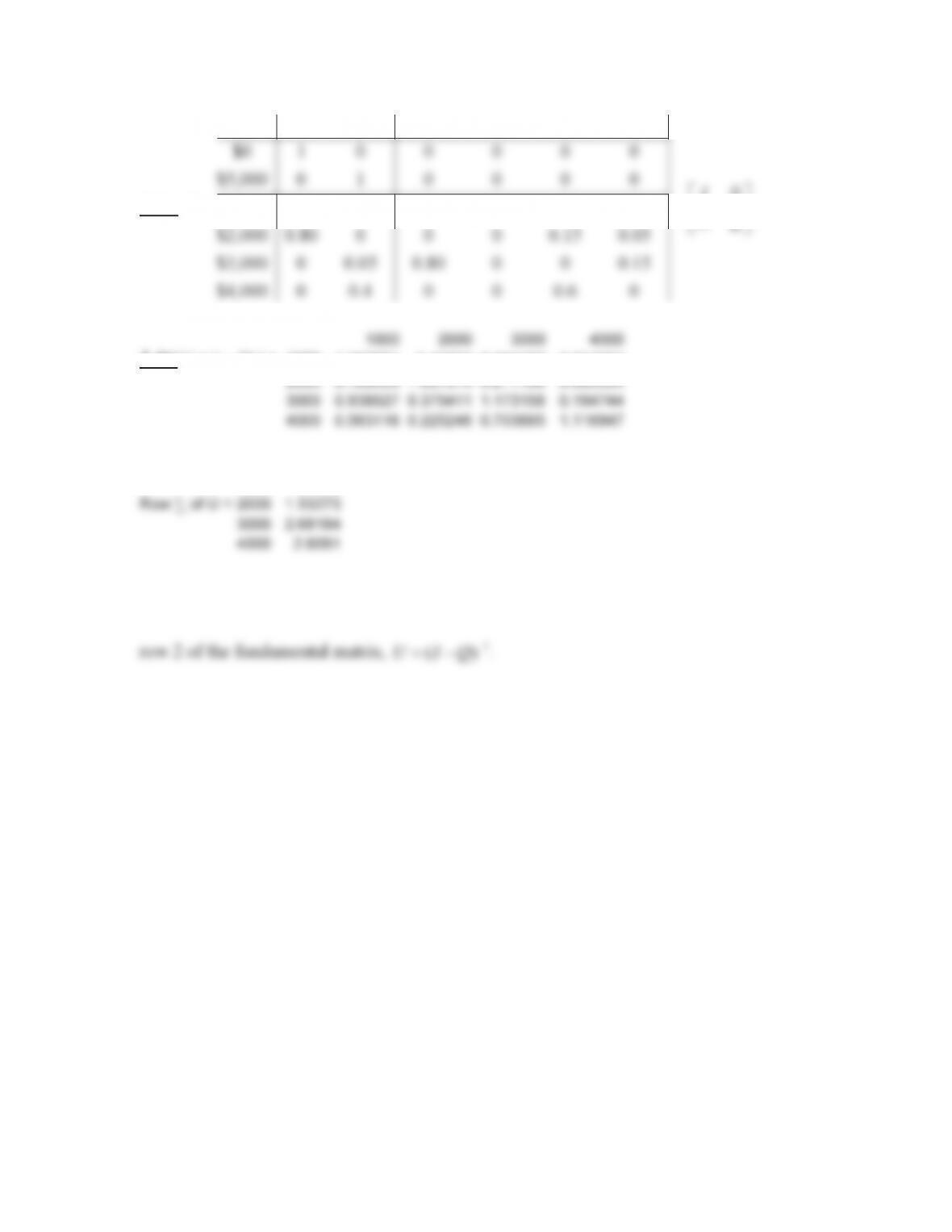
State $0 $5,000 $1,000 $2,000 $3,000 $4,000
$1,000 0.6 0 0 0.4 0 0
I
PDQ
ªº
«»
1000
2000
3000
4000
3.4b) U = (I – Q)-1 = 1000
1.067574
0.42703
0.084467
0.034022
2000
0.168935
1.067574
0.211168
0.085054
3000
0.938527
0.375411
1.173158
0.194744
4000
0.563116
0.225246
0.703895
1.116847
1000
1.61309
Row ∑ of U = 2000
1.53273
3000
2.68184
4000
2.6091
The expected number of bets that she will make equals 1.53273, the sum of the entries in
1
28
0
5000
3.4c) F = UD = (I – Q)
-1
D = 1000
0.98217
0.01783
2000
0.95542
0.04458
3000
0.86344
0.13656
4000
0.51807
0.48193
P (that she will obtain her $5,000 down payment)
2000, 5000
3.5)
3.5a)
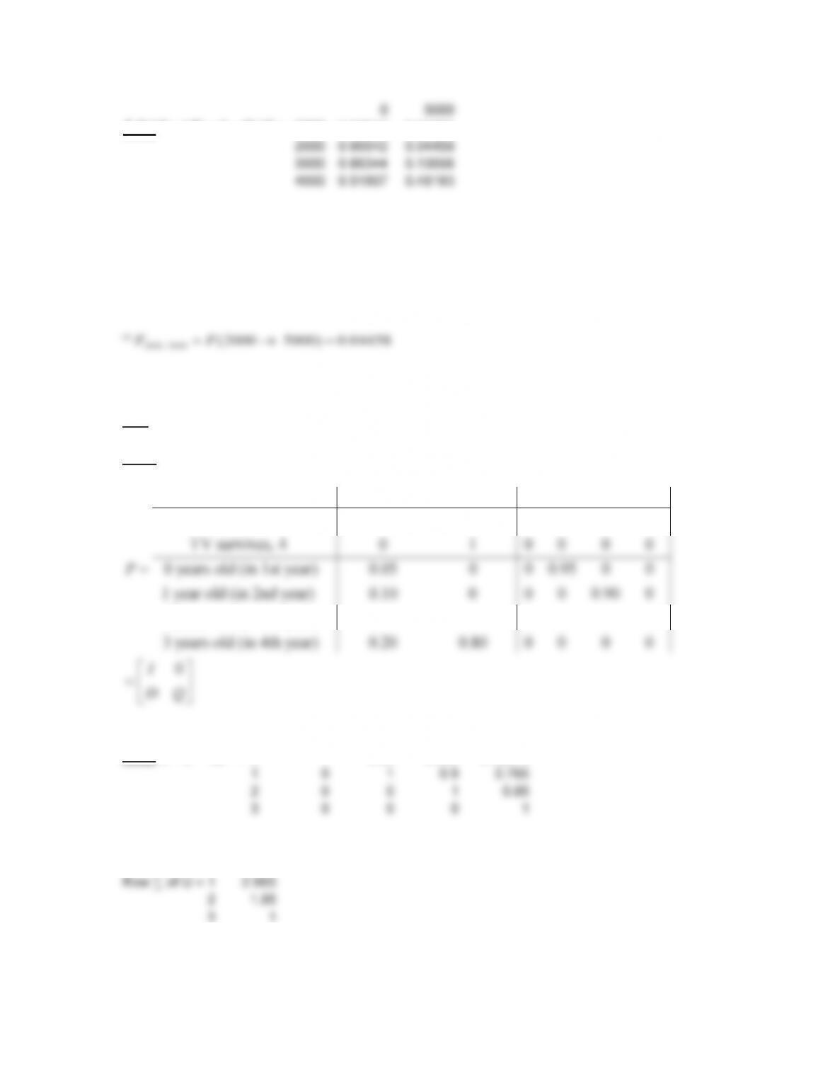
State Replaced, 5 Survives, 4 0 1 2 3
TV fails and is replaced, 5 1 0 0 0 0 0
2 years old (in 3rd year) 0.15 0 0 0 0 0.85
3
years old (in 4th year) 0.20 0.80 0 0 0 0
0I
DQ
ªº
«»
¬¼
0
1
2
3
3.5b) U = (I – Q)-1 = 0
1
0.95
0.855
0.72675
1
0
1
0.9
0.765
2
0
0
1
0.85
3
0
0
0
1
0
3.53175
Row ∑ of U = 1
2.665
2
1.85
3
1
29
5
4
F = UD = (I – Q)
-1
D = 0
0.4186
0.5814
1
0.388
0.612
2
0.32
0.68
3
0.2
0.8
05
3.5c) The dealer’s expected revenue from selling a 4–year warranty
05
3.6)
State 5, Scrapped 4, Sold 1 2 3
1, Stage 1 0.08 0 0.12 0.80 0
P
¬¼
1
2
3
3.6b) U = (I – Q)
-1
= 1
1.136364
0.999001
0.903352
2
0
1.098901
0.993687
3
0
0
1.06383
1
3.038717
Row ∑ of U = 2
2.092588
3
1.06383
5
4
F = UD = (I – Q)
-1
D = 1
0.18698
0.81302
2
0.10568
0.89432
3
0.04255
0.95745
30
P(an item will be scrapped before it can be sold, given that it is in stage 3)
0.04255f
.
12 23 34
3.6d) P(an item will be in stage 2 after 3 inspections)
(3)
14
3.6g) Mean number of inspections that an item will receive in stage 3
3.6h) Given that an item is in stage 2, the mean number of inspections that it will receive
3.7)
3.7a)
State 1 2 5 3 4
2, On course to LEO 0 1 0 0 0 0
I
PDQ
ªº
3
4
3.7b) U = (I – Q)
-1
= 3
1.13475
0.070922
4
0.42553
1.276596
3
1.205674
Row ∑ of U = 4
1.702128
31
1
2
5
F = UD = (I – Q)
-1
D = 3
0.624113
0.368794
0.00709
4
0.234043
0.638298
0.12766
3.7d)
][
)0(
5
)0(
4
)0(
3
)0(
2
)0(
1
)0(
pppppp
]02.08.000[
0.8 0.2ff
0.8(0.6241) + 0.2(0.2340) = 0.5461
= 0.021
3.8)
3.8a)
»
»
¼
«
«
¬
»
»
¼
«
«
¬
pr
QI
pr
Q
10
)(,
0
1
»
º
«
ª
pr
01
»
»
»
»
º
«
«
«
«
ª
pd
p
pd
p
pd
p
pd
00
1
)()(
1
3
2
2
100
001
ªº
«»
«»
¬¼
32
3.8b) Letting
pd
p
t
,
»
º
«
ª
1
2
tt
dp
3.8e)
45
10
20
d
Dd
ªº
«»
«»
1
)1(
2
º
ª
rtdtd
3.8g)
12 11 12 12 22
2ppppprpprpr
3.9)
3.0002.01.04.0professor Associate3
2.03.00005.0professorAssistant 2
000001Discharged6
321546`State
1
2
3
1
1.428571
0.204082
0.058309
1
()UIQ
= 2
0
1.428571
0.408163
3
0
0
1.428571
6
1
0.98251
34
23 22 23 23 33
3.9f) Using the results of Section 3.5.5.1, the limiting transition probability matrix is
45
1 0 0 000
6
0 000
4
SS
ªº
«»
For
,
6
4
5
1
2
3
fo
n
n
Plim
6
1
0
0
0
0
0
4
0
0.4
0.6
0
0
0
5
0
0.4
0.6
0
0
0
1
0.9825
0.007
0.0105
0
0
0
2
0.8776
0.049
0.0735
0
0
0
3
0.5714
0.1714
0.2571
0
0
0
=
()ff
S
= 0.2571
5
3.10)
3.10a)
»
¼
«
¬
QD
P0
24.040.020.006.010.015
14.030.024.010.022.010
20.032.028.008.00.125
000010
15105200State
5
10
15
5
2.085963
1.416351
0.809844
3.10b)
1
()UIQ
= 10
0.922031
2.22269
0.652082
15
1.034217
1.542561
1.872108
5
4.312158
Row ∑ of U = 10
3.796803
15
4.448885
0
20
5
0.6429
0.3571