Applied Statistics and Probability for Engineers, 7th edition 2017
15-1
CHAPTER 15
Section 15-3
15.3.1 Control charts are to be constructed for samples of size n = 4, and x and s are computed for each of 20 preliminary
samples as follows:
=
=
20
1
4460
i
i
x
=
=
20
1
271.6
i
i
s
(a) Calculate trial control limits for
X
and S charts.
(b) Assuming the process is in control, estimate the process mean and standard deviation.
(a)
==
4460 223
20
x
==
271.6 13.58
20
s
15.3.2 Twenty-five samples of size 5 are drawn from a process at one-hour intervals, and the following data are obtained:
=
=
25
1
362.75
i
i
x
=
=
25
1
8.60
i
i
r
=
=
25
1
3.64
i
i
s
(a) Calculate trial control limits for
X
and R charts.
(b) Repeat part (a) for
X
and S charts.
Applied Statistics and Probability for Engineers, 7th edition 2017
15-2
15.3.3 The level of cholesterol (in mg/dL) is an important index for human health. The sample size is n = 5. The following
summary statistics are obtained from cholesterol measurements:
=
=
30
1
140.03
i
i
x
=
=
30
1
13.63
i
i
r
=
=
30
1
5.10
i
i
s
(a) Find trial control limits for
X
and R charts.
(b) Repeat part (a) for
X
and S charts.
(b)
==
5.10 0.17
30
s
Applied Statistics and Probability for Engineers, 7th edition 2017
15-3
15.3.4 An
X
control chart with three-sigma control limits has UCL = 48.75 and LCL = 42.71.
Suppose that the process standard deviation is
= 2.25. What subgroup size was used for the chart?
For the
x
chart:
15.3.5 The pull strength of a wire-bonded lead for an integrated circuit is monitored. The following table provides data for 20
samples each of size 3.
Sample Number
x1
x2
x3
1
15.4
15.6
15.3
2
15.4
17.1
15.2
3
16.1
16.1
13.5
4
13.5
12.5
10.2
5
18.3
16.1
17.0
6
19.2
17.2
19.4
7
14.1
12.4
11.7
8
15.6
13.3
13.6
9
13.9
14.9
15.5
10
18.7
21.2
20.1
11
15.3
13.1
13.7
12
16.6
18.0
18.0
13
17.0
15.2
18.1
14
16.3
16.5
17.7
15
8.4
7.7
8.4
16
11.1
13.8
11.9
17
16.5
17.1
18.5
18
18.0
14.1
15.9
19
17.8
17.3
12.0
20
11.5
10.8
11.2
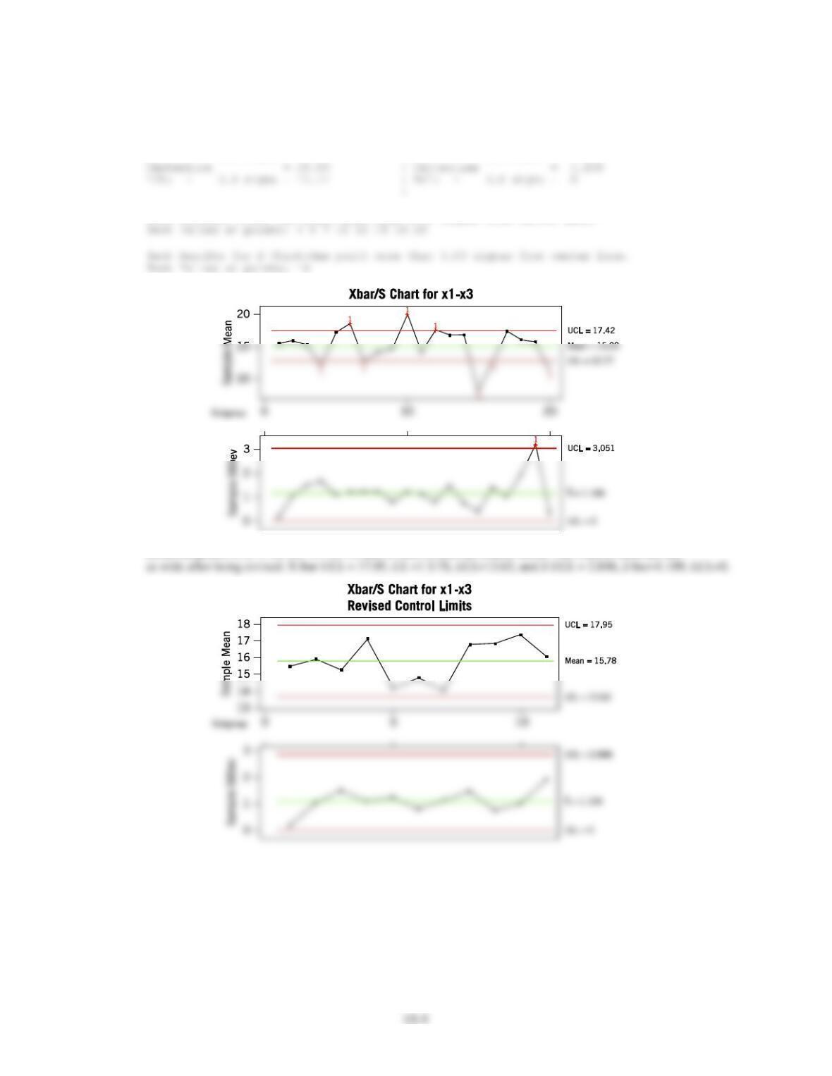
(a) Use all the data to determine trial control limits for
X
and R charts, construct the control limits, and plot
the data.
(b) Use the control limits from part (a) to identify out-of-control points. If necessary, revise your control limits
assuming that any samples that plot outside of the control limits can be eliminated.
(c) Repeat parts (a) and (b) for
X
and S charts.
Applied Statistics and Probability for Engineers, 7th edition 2017
15-4
(a) X–bar and Range – Initial Study
Charting Problem 15-9
X-bar | Range
|
Test Results: X-bar One point more than 3.00 sigmas from center line.
(b) Removed points 4, 6, 7, 10, 12, 15, 16, 19, and 20 and revised the control limits. The control limits are not as wide after
Applied Statistics and Probability for Engineers, 7th edition 2017
(c) X–bar and StDev – Initial Study
Charting Problem 16-7
X-bar | StDev
—– | —–
UCL: + 3.0 sigma = 17.42 | UCL: + 3.0 sigma = 3.051
Test Results: X-bar One point more than 3.00 sigmas from center line.
Removed points 4, 6, 7, 10, 12, 15, 16, 19, and 20 and revised the control limits. The control limits are not
15.3.6 The copper content of a plating bath is measured three times per day, and the results are reported in ppm. The
x
and r
values for 25 days are shown in the following table:
Day
x
r
Day
x
r
1
5.45
1.21
14
7.01
1.45
2
5.39
0.95
15
5.83
1.37
3
6.85
1.43
16
6.35
1.04
4
6.74
1.29
17
6.05
0.83
5
5.83
1.35
18
7.11
1.35
6
7.22
0.88
19
7.32
1.09
7
6.39
0.92
20
5.90
1.22
8
6.50
1.13
21
5.50
0.98
9
7.15
1.25
22
6.32
1.21
10
5.92
1.05
23
6.55
0.76
11
6.45
0.98
24
5.90
1.20
12
5.38
1.36
25
5.95
1.19
13
6.03
0.83
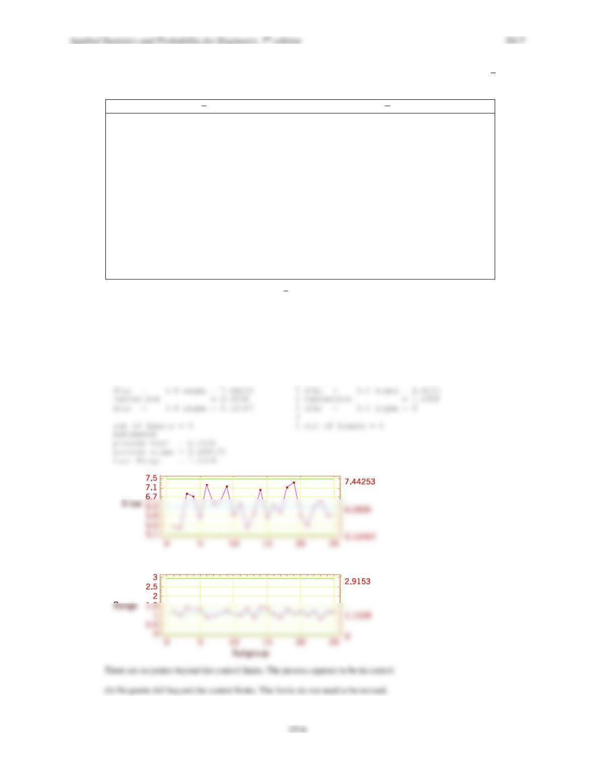
(a) Using all the data, find trial control limits for
X
and R charts, construct the chart, and plot the data. Is the process
in statistical control?
(b) If necessary, revise the control limits computed in part (a), assuming that any samples that plot outside the control
limits can be eliminated.
(a)
X-bar and Range – Initial Study
Charting Problem 15-8
X-bar | Range
—– | —–
15-7
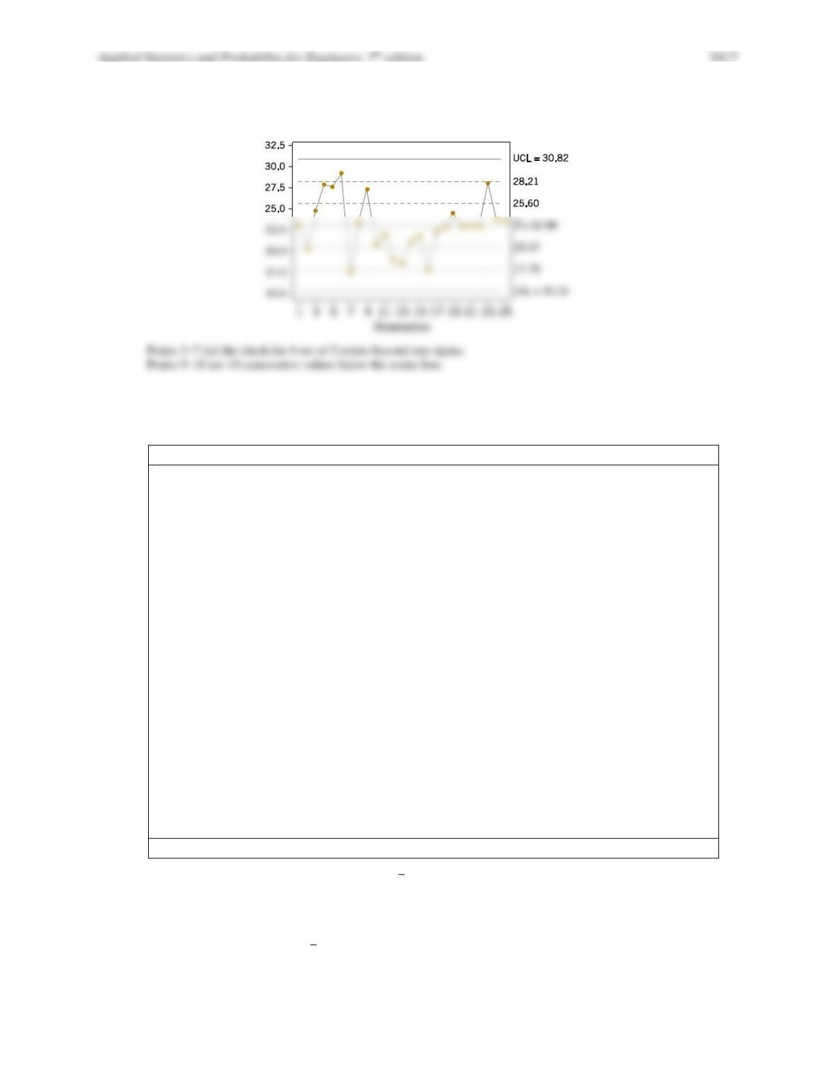
15.3.7 Apply the Western Electric Rules to the following control chart. The warning limits are shown as dotted lines. Describe
any rule violations.
15.3.8 The following data were considered in Quality Engineering [“An SPC Case Study on Stabilizing Syringe Lengths”
(1999–2000, Vol. 12(1))]. The syringe length is measured during a pharmaceutical manufacturing process. The
following table provides data (in inches) for 20 samples each of size 5.
Sample
x1
x2
x3
x4
x5
1
4.960
4.946
4.950
4.956
4.958
2
4.958
4.927
4.935
4.940
4.950
3
4.971
4.929
4.965
4.952
4.938
4
4.940
4.982
4.970
4.953
4.960
5
4.964
4.950
4.953
4.962
4.956
6
4.969
4.951
4.955
4.966
4.954
7
4.960
4.944
4.957
4.948
4.951
8
4.969
4.949
4.963
4.952
4.962
9
4.984
4.928
4.960
4.943
4.955
10
4.970
4.934
4.961
4.940
4.965
11
4.975
4.959
4.962
4.971
4.968
12
4.945
4.977
4.950
4.969
4.954
13
4.976
4.964
4.970
4.968
4.972
14
4.970
4.954
4.964
4.959
4.968
15
4.982
4.962
4.968
4.975
4.963
16
4.961
4.943
4.950
4.949
4.957
17
4.980
4.970
4.975
4.978
4.977
18
4.975
4.968
4.971
4.969
4.972
19
4.977
4.966
4.969
4.973
4.970
20
4.975
4.967
4.969
4.972
4.972
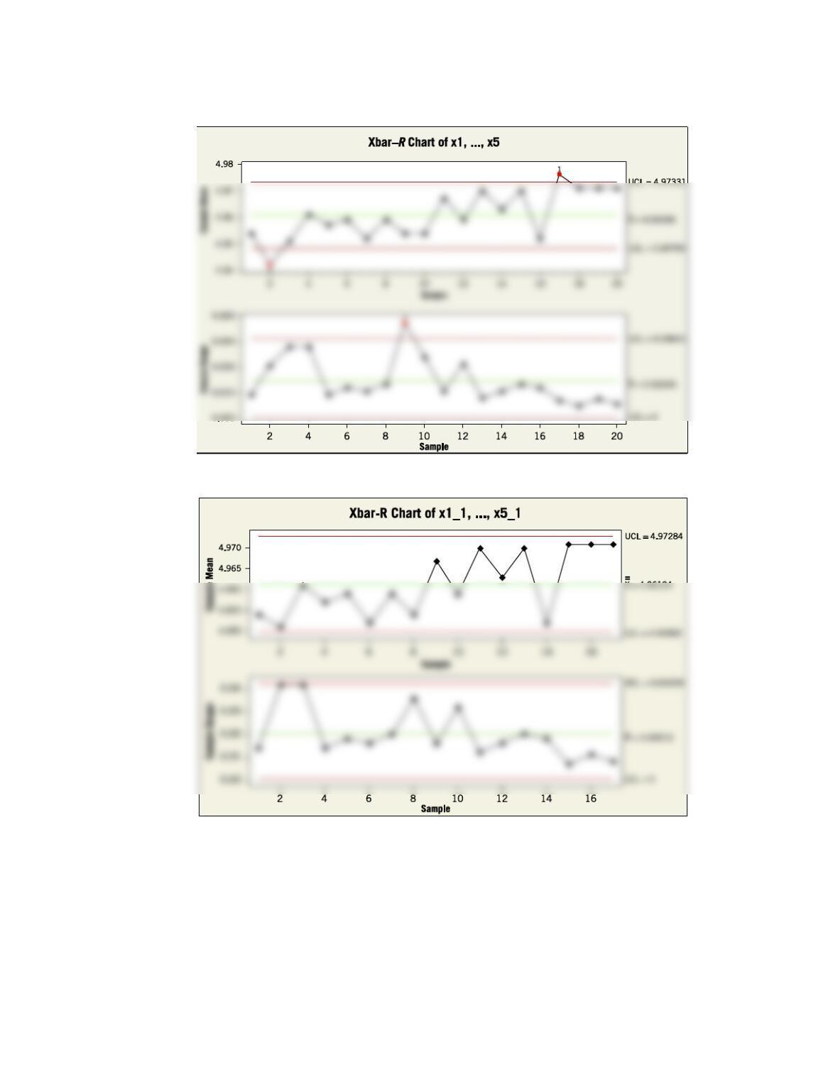
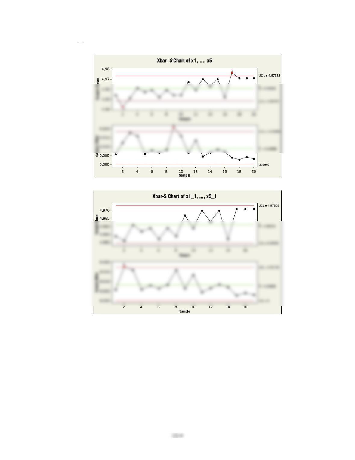
(a) Using all the data, find trial control limits for
X
and R charts, construct the chart, and plot the data. Is this process
in statistical control?
(b) Use the trial control limits from part (a) to identify out-of-control points. If necessary, revise your control limits
assuming that any samples that plot outside the control limits can be eliminated.
(c) Repeat parts (a) and (b) for
X
and S charts.
Applied Statistics and Probability for Engineers, 7th edition 2017
15-8
(a) The average range is used to estimate the standard deviation. Samples 2, 9, and 17 are out-of-control.
(b)
Applied Statistics and Probability for Engineers, 7th edition 2017
(c) For
X
–S chart
15–10
15.3.9 Consider the data in Exercise 15.3.5 Calculate the sample standard deviation of all 60 measurements and compare this
result to the estimate of obtained from your revised
X
and R charts. Explain any differences.
15.3.10 Web traffic can be measured to help highlight security problems or indicate a potential lack of bandwidth. Data on Web
traffic (in thousand hits) from http://en.wikipedia.org/wiki/Web_traffic are given in the following table for 25 samples
each of size 4.
Sample
x1
x2
x3
x4
1
163.95
164.54
163.87
165.10
2
163.30
162.85
163.18
165.10
3
163.13
165.14
162.80
163.81
4
164.08
163.43
164.03
163.77
5
165.44
163.63
163.95
164.78
6
163.83
164.14
165.22
164.91
7
162.94
163.64
162.30
163.78
8
164.97
163.68
164.73
162.32
9
165.04
164.06
164.40
163.69
10
164.74
163.74
165.10
164.32
11
164.72
165.75
163.07
163.84
12
164.25
162.72
163.25
164.14
13
164.71
162.63
165.07
162.59
14
166.61
167.07
167.41
166.10
15
165.23
163.40
164.94
163.74
16
164.27
163.42
164.73
164.88
17
163.59
164.84
164.45
164.12
18
164.90
164.20
164.32
163.98
19
163.98
163.53
163.34
163.82
20
164.08
164.33
162.38
164.08
21
165.71
162.63
164.42
165.27
22
164.03
163.36
164.55
165.77
23
160.52
161.68
161.18
161.33
24
164.22
164.27
164.35
165.12
25
163.93
163.96
165.05
164.52
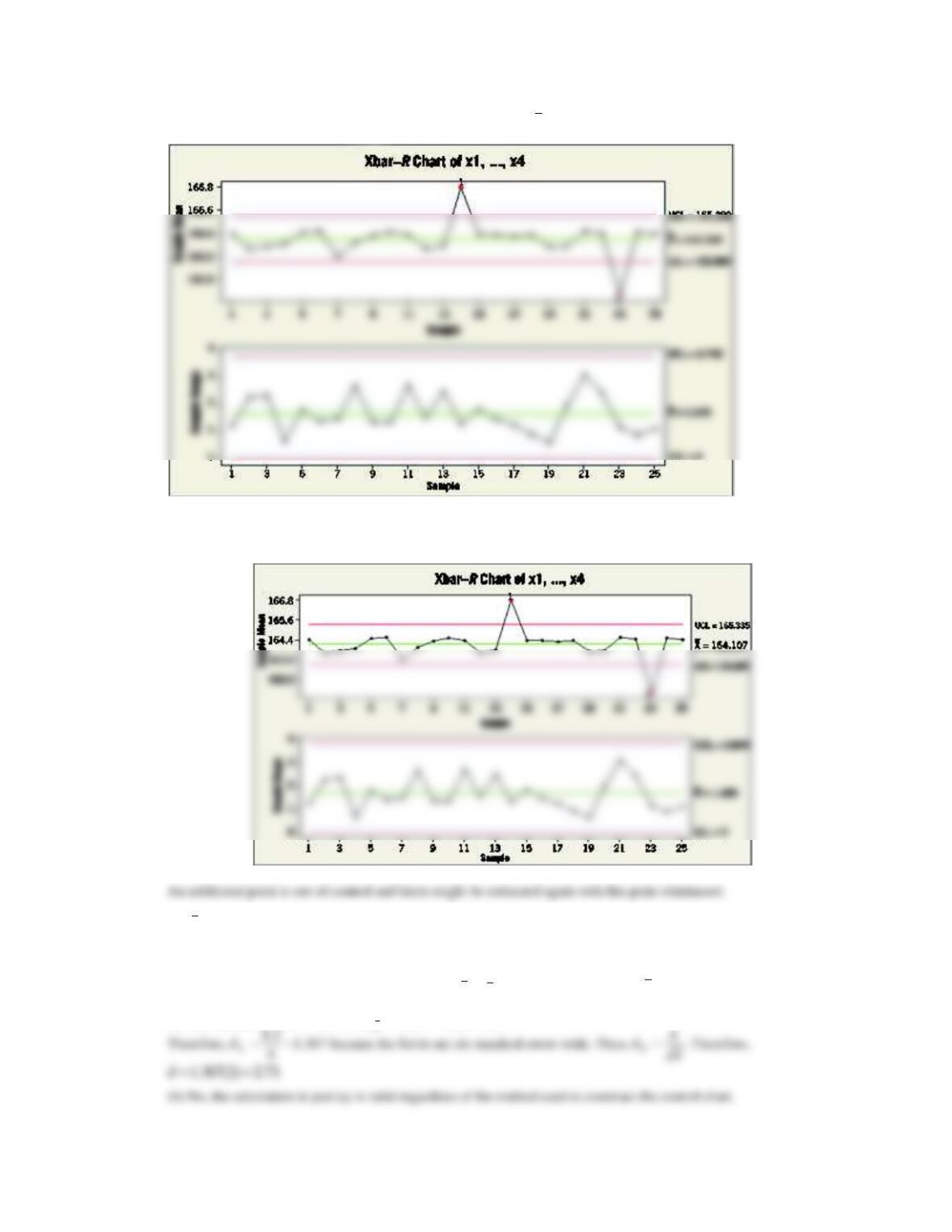
(a) Use all the data to determine trial control limits for
X
and R charts, construct the chart, and plot the data.
(b) Use the trial control limits from part (a) to identify out-of-control points. If necessary, revise your control limits,
assuming that any samples that plot outside the control limits can be eliminated.
Applied Statistics and Probability for Engineers, 7th edition 2017
15–11
(a) The control limits for the following chart were obtained from
R
.
(b) The test failed at points 14 and 23. The control limits are revised by omitting the out-of-control points from the
control limit calculations.
15.3.11 An
X
control chart with 3-sigma control limits and subgroup size n = 4 has control limits UCL = 48.75 and
LCL = 40.55.
(a) Estimate the process standard deviation.
(b) Does the response to part (a) depend on whether
r
or
s
was used to construct the
X
control chart?
(a) The difference
− = = − =
ˆ
6 48.75 40.55 8.2
X
UCL LCL
Applied Statistics and Probability for Engineers, 7th edition 2017
15–12
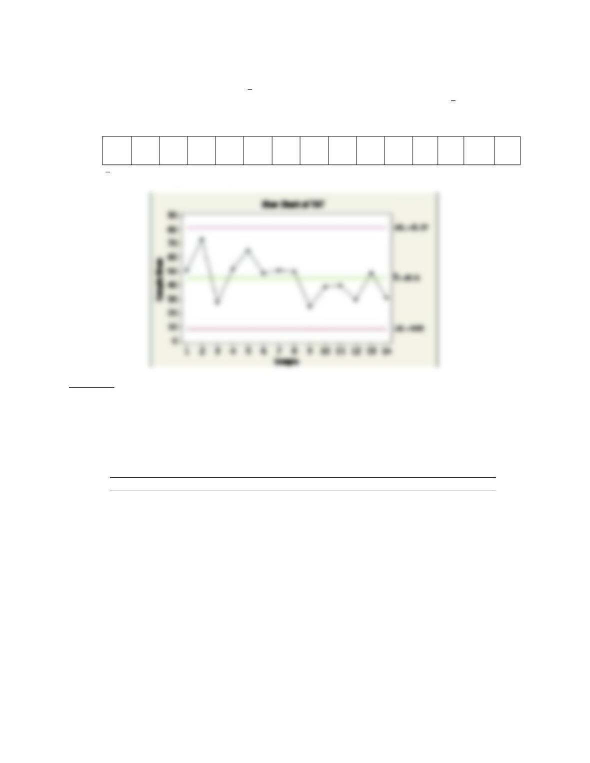
15.3.12 An article in Quality & Safety in Health Care [“Statistical Process Control as a Tool for Research and Healthcare
Improvement,” (2003) Vol. 12, pp. 458–464] considered a number of control charts in healthcare. The following
approximate data were used to construct
−XS
charts for the turnaround time (TAT) for complete blood counts (in
minutes). The subgroup size is n = 3 per shift, and the mean standard deviation is 21. Construct the
X
chart and
comment on the control of the process. If necessary, assume that assignable causes can be found, eliminate suspect
points, and revise the control limits.
t
1
2
3
4
5
6
7
8
9
10
11
12
13
14
TAT
51
73
28
52
65
49
51
50
25
39
40
30
49
31
−XS
chart, and the process is in control.
Section 15-4
15.4.1 In a semiconductor manufacturing process, CVD metal thickness was measured on 30 wafers obtained over
approximately two weeks. Data are shown in the following table.
(a) Using all the data, compute trial control limits for individual observations and moving-range charts. Construct the
chart and plot the data. Determine whether the process is in statistical control. If not, assume that assignable
causes can be found to eliminate these samples and revise the control limits.
(b) Estimate the process mean and standard deviation for the in-control process.
Wafer
x
Wafer
x
1
16.8
16
15.4
2
14.9
17
14.3
3
18.3
18
16.1
4
16.5
19
15.8
5
17.1
20
15.9
6
17.4
21
15.2
7
15.9
22
16.7
8
14.4
23
15.2
9
15.0
24
14.7
10
15.7
25
17.9
11
17.1
26
14.8
12
15.9
27
17.0
13
16.4
28
16.2
14
15.8
29
15.6
15
15.4
30
16.3
Applied Statistics and Probability for Engineers, 7th edition 2017
15–13
(a) The process appears to be in statistical control. There are no points beyond the control limits.
(b) Estimated process mean and standard deviation
15.4.2 The viscosity of a chemical intermediate is measured every hour. Twenty samples each of size n = 1 are in the
following table.
Sample
Viscosity
Sample
Viscosity
1
495
11
493
2
491
12
507
3
501
13
503
4
501
14
475
5
512
15
497
6
540
16
499
7
492
17
468
8
504
18
486
9
542
19
511
10
508
20
487
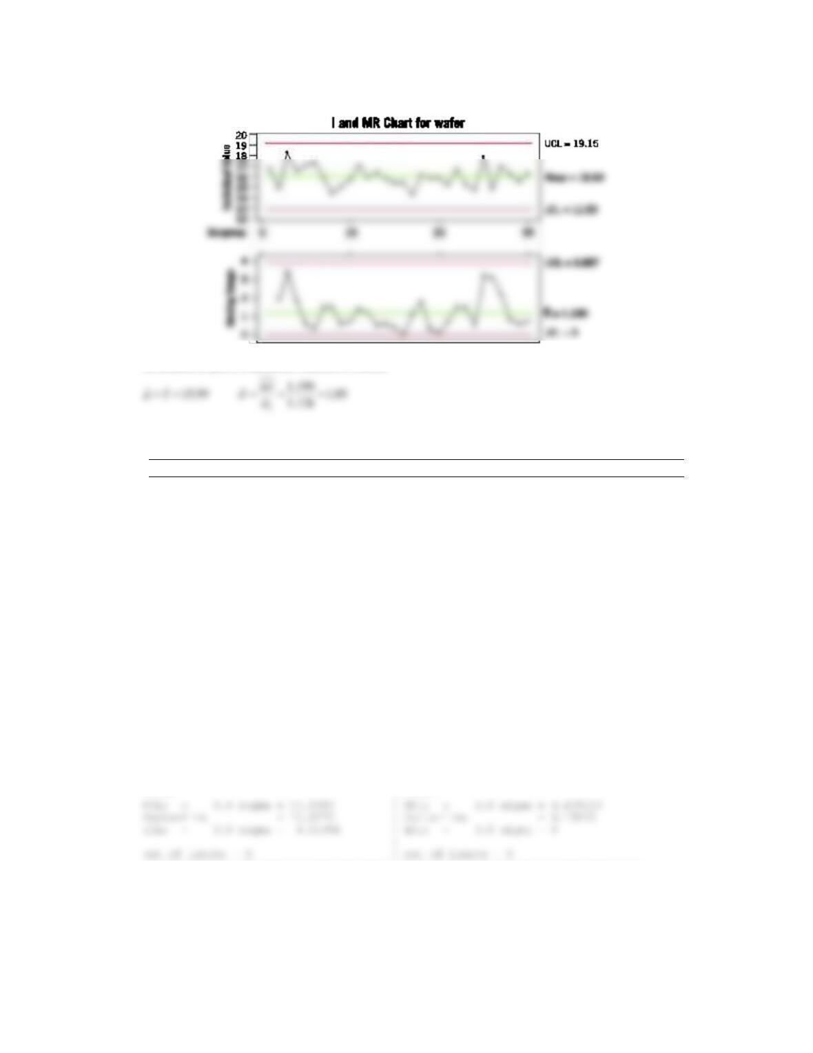
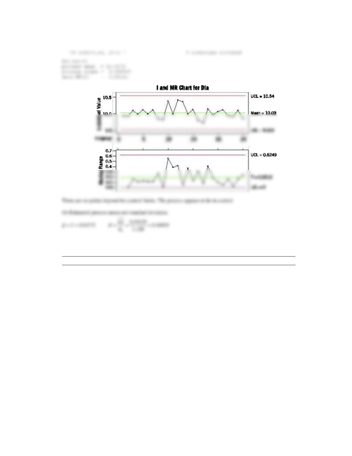
(a) Using all the data, compute trial control limits for individual observations and moving-range charts. Determine
whether the process is in statistical control. If not, assume that assignable causes can be found to eliminate these
samples and revise the control limits.
(b) Estimate the process mean and standard deviation for the in-control process.
(a) Ind.x and MR(2) – Initial Study
——————————————————————————
Charting diameter
Ind.x | MR(2)
——————————————————————————
Applied Statistics and Probability for Engineers, 7th edition 2017
15–14
Chart: Both Normalize: No
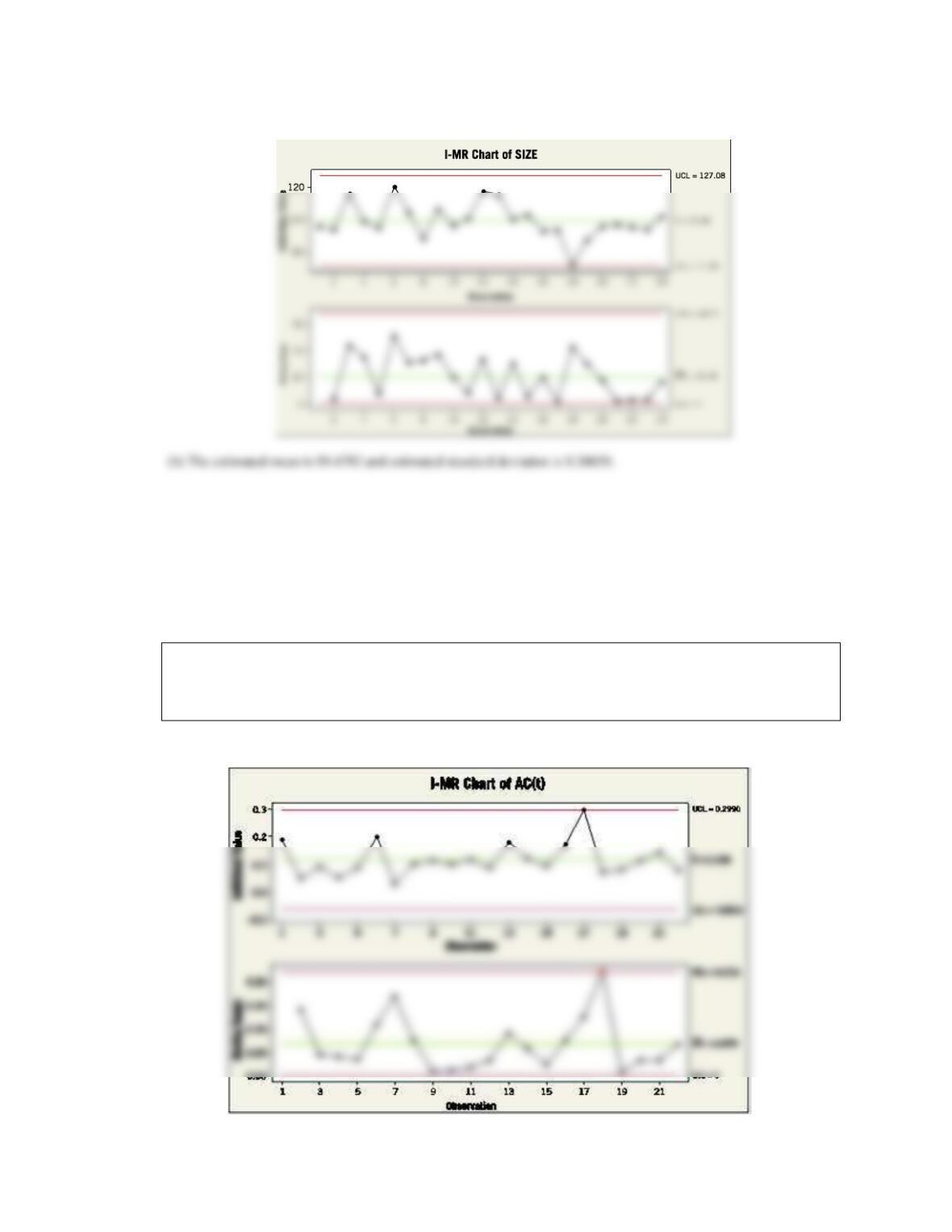
15.4.3 The following table of data was analyzed in Quality Engineering [1991–1992, Vol. 4(1)]. The average particle size of
raw material was obtained from 25 successive samples.
Observation
Size
Observation
Size
1
96.1
14
100.5
2
94.4
15
103.1
3
116.2
16
93.1
4
98.8
17
93.7
5
95.0
18
72.4
6
120.3
19
87.4
7
104.8
20
96.1
8
88.4
21
97.1
9
106.8
22
95.7
10
96.8
23
94.2
11
100.9
24
102.4
12
117.7
25
131.9
13
115.6
(a) Using all the data, compute trial control limits for individual observations and moving-range charts. Construct the
chart and plot the data. Determine whether the process is in statistical control. If not, assume that assignable
causes can be found to eliminate these samples and revise the control limits.
(b) Estimate the process mean and standard deviation for the in-control process.
Applied Statistics and Probability for Engineers, 7th edition 2017
15–15
(a) The process is out of control. The control charts follow.
Remove the out-of-control observation 25:
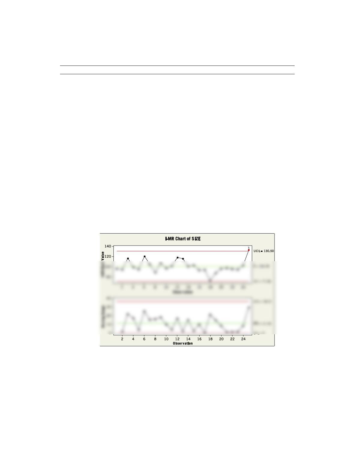
Applied Statistics and Probability for Engineers, 7th edition 2017
15–16
15.4.4 Pulsed laser deposition technique is a thin film deposition technique with a high-powered laser beam.
Twenty-five films were deposited through this technique. The thicknesses of the films obtained are shown in
the following table.
Film
Thickness (nm)
Film
Thickness (nm)
1
28
8
51
2
45
9
23
3
34
10
35
4
29
11
47
5
37
12
50
6
52
13
32
7
29
14
40
15
46
21
21
16
59
22
62
17
20
23
34
18
33
24
31
19
56
25
98
20
49
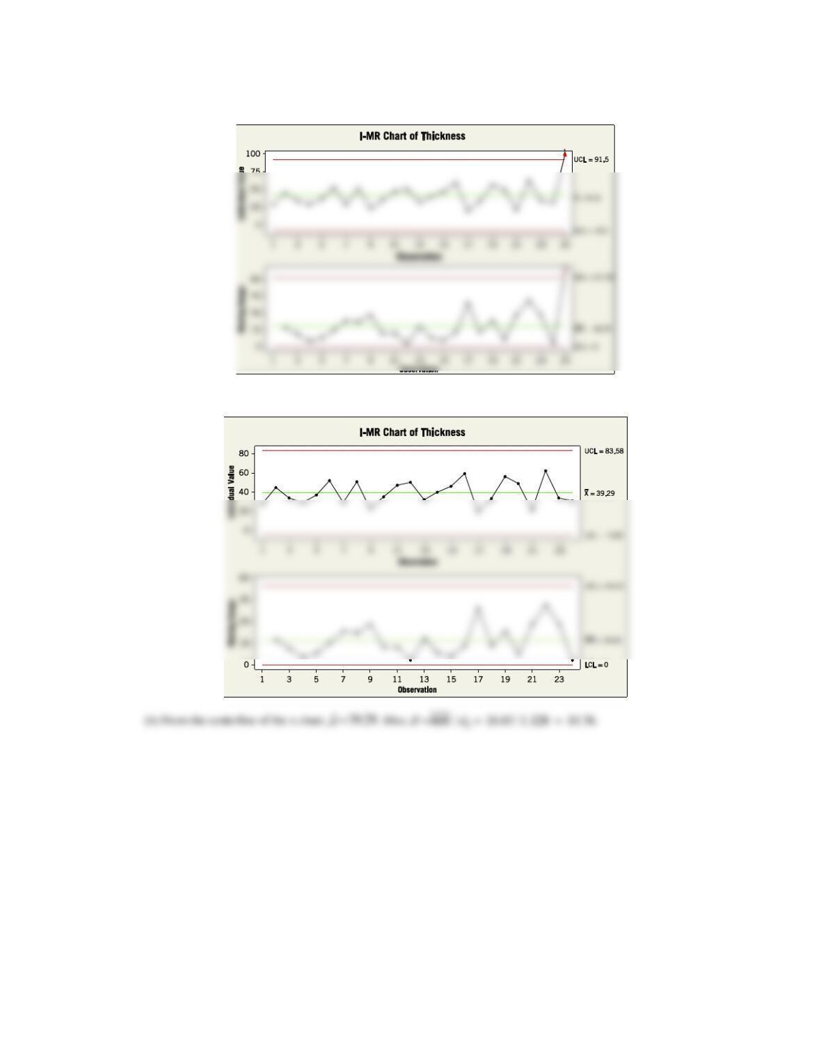
(a) Using all the data, compute trial control limits for individual observations and moving-range charts. Determine
whether the process is in statistical control. If not, assume that assignable causes can be found to eliminate these
samples, and revise the control limits.
(b) Estimate the process mean and standard deviation for the in-control process.
(a)
Applied Statistics and Probability for Engineers, 7th edition 2017
15–17
Remove the out-of-control observation:
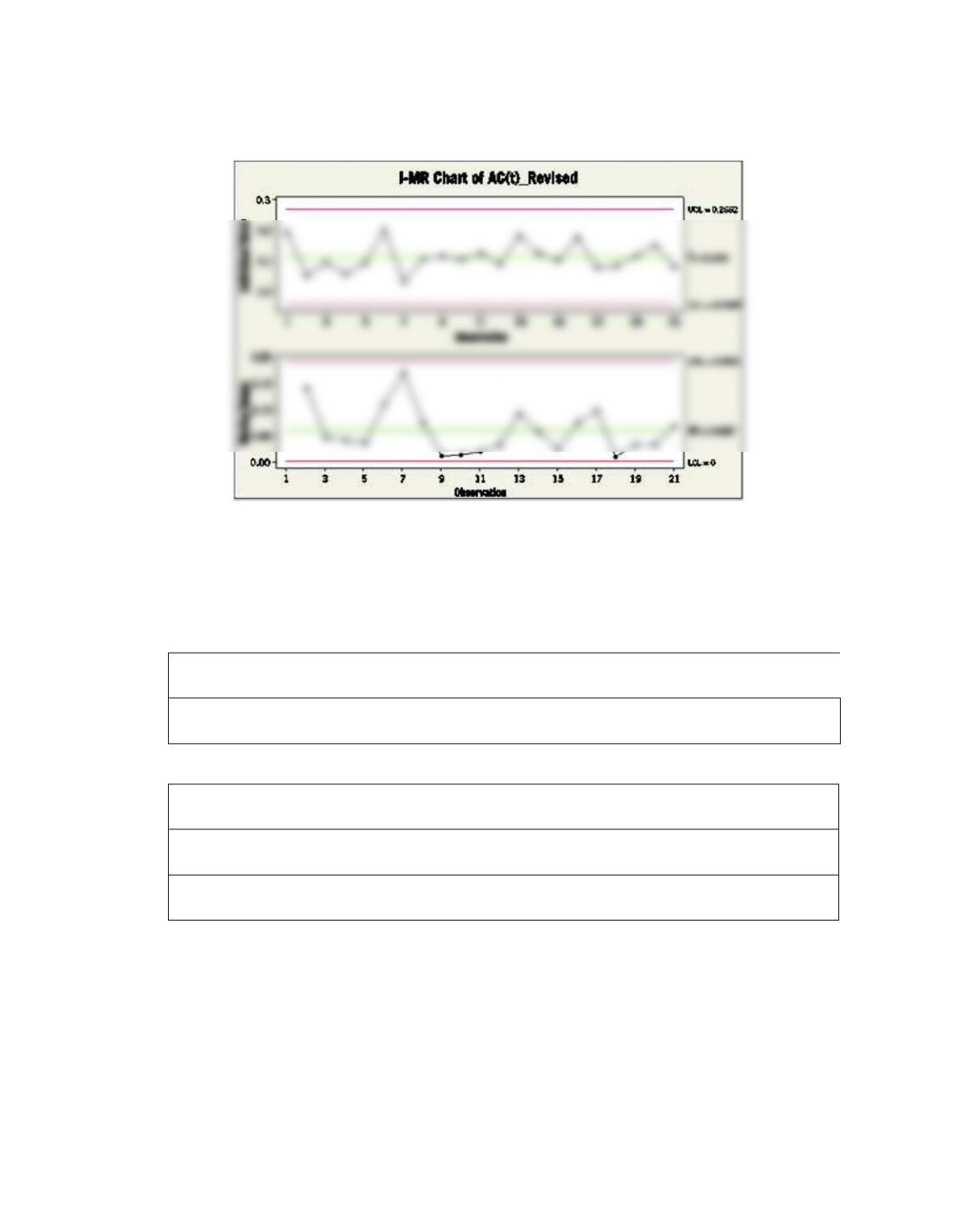
15.4.5 An article in Journal of the Operational Research Society [“A Quality Control Approach for Monitoring Inventory
Stock Levels,” (1993, pp. 1115–1127)] reported on a control chart to monitor the accuracy of an inventory management
system. Inventory accuracy at time t, AC(t), is defined as the difference between the recorded and actual inventory (in
absolute value) divided by the recorded inventory. Consequently, AC(t) ranges between 0 and 1 with lower values
better. Extracted data are shown in the following table.
(a) Calculate individuals and moving-range charts for these data.
(b) Comment on the control of the process. If necessary, assume that assignable causes can be found, eliminate
suspect points, and revise the control limits.
t
1
2
3
4
5
6
7
8
9
10
11
AC(t)
0.190
0.050
0.095
0.055
0.090
0.200
0.030
0.105
0.115
0.103
0.121
t
12
13
14
15
16
17
18
19
20
21
22
AC(t)
0.089
0.180
0.122
0.098
0.173
0.298
0.075
0.083
0.115
0.147
0.079
(a) Individuals and moving range charts follow.
Applied Statistics and Probability for Engineers, 7th edition 2017
15–18
(b) There is an out of control point on the moving range chart (|observation 18-observation 17| with moving range
0.223). Remove the suspect point (observation 17) and re-do the analysis.
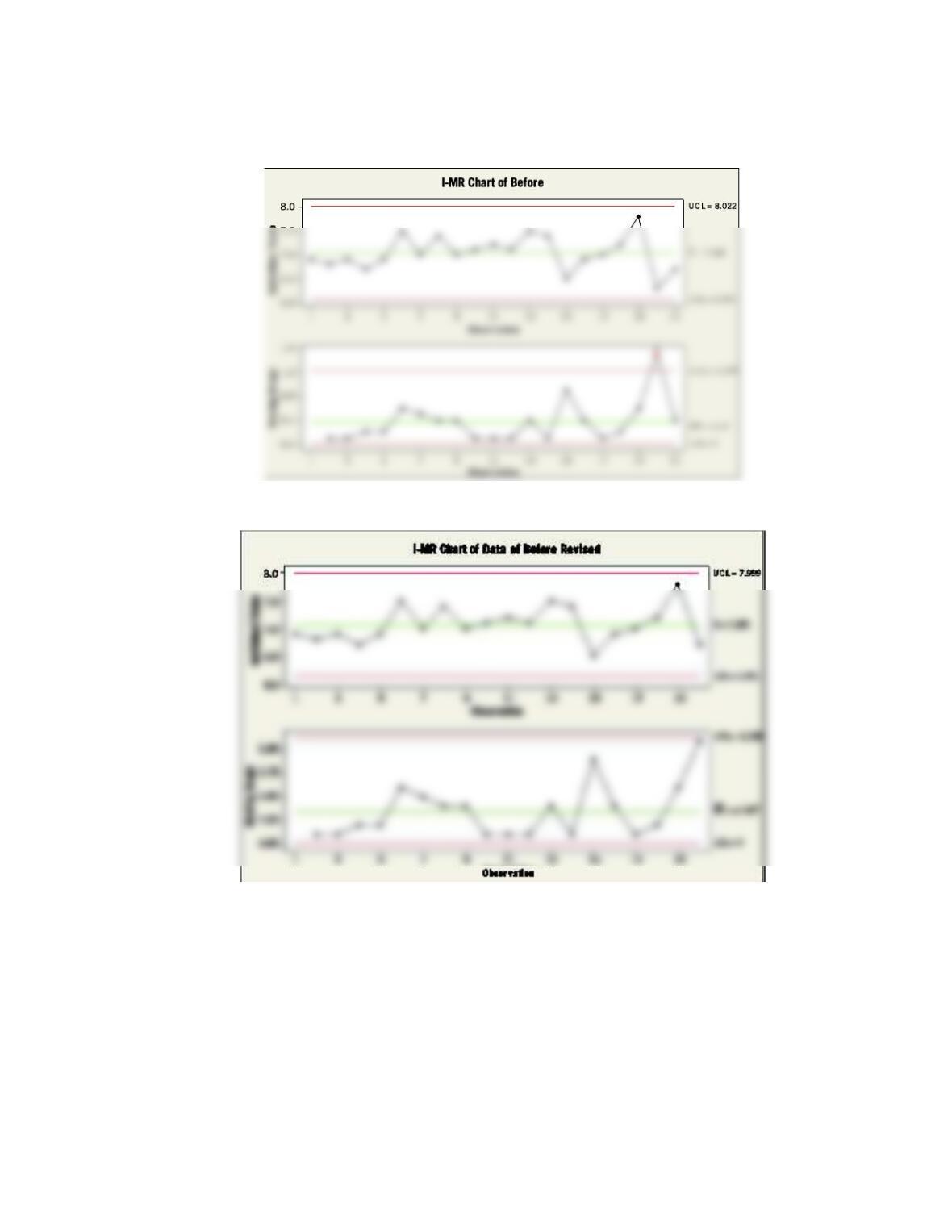
15.4.6 An article in Quality & Safety in Health Care [“Statistical Process Control as a Tool for Research and Healthcare
Improvement,” (2003 Vol. 12, pp. 458–464)] considered a number of control charts in healthcare. An X chart was
constructed for the amount of infectious waste discarded each day (in pounds). The article mentions that improperly
classified infectious waste (actually not hazardous) adds substantial costs to hospitals each year. The following tables
show approximate data for the average daily waste per month before and after process changes, respectively. The
process change included an education campaign to provide an operational definition for infectious waste.
Before Process Change
Month
1
2
3
4
5
6
7
8
9
Waste
6.9
6.8
6.9
6.7
6.9
7.5
7
7.4
7
Month
13
14
15
16
17
18
19
20
21
Waste
7.5
7.4
6.5
6.9
7.0
7.2
7.8
6.3
6.7
After Process Change
Month
1
2
3
4
5
6
7
8
9
10
11
12
Waste
5.0
4.8
4.4
4.3
4.6
4.3
4.5
3.5
4.0
4.1
3.8
5.0
Month
13
14
15
16
17
18
19
20
21
22
23
24
Waste
4.6
4.0
5.0
4.9
4.9
5.0
6.0
4.5
4.0
5.0
4.5
4.6
Month
25
26
27
28
29
30
Waste
4.6
3.8
5.3
4.5
4.4
3.8
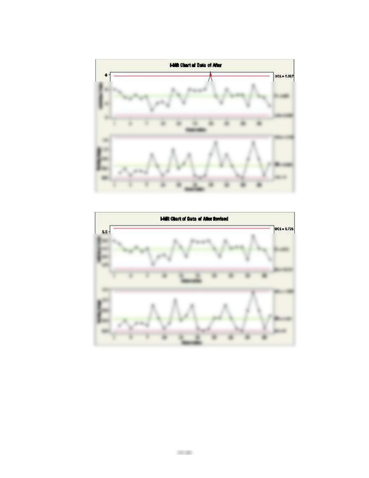
(a) Handle the data before and after the process change separately and construct individuals and moving-range charts
for each set of data. Assume that assignable causes can be found and eliminate suspect observations. If necessary,
revise the control limits.
(b) Comment on the control of each chart and differences between the charts. Was the process change effective?
Applied Statistics and Probability for Engineers, 7th edition 2017
15–19
(a) For data before the process change, point 20 on the moving range chart is more than 3 standard deviations from
center line.
Assume the assignable cause can be found and eliminate point 20 and revise the control chart.
Applied Statistics and Probability for Engineers, 7th edition 2017
For data of after process change, point 19 on the individuals chart is more than 30 standard deviations from the
centerline.
Assume the assignable cause can be found and eliminate point 19 and revise the control chart.