15–41
15.8.4 The concentration of a chemical product is measured by taking four samples from each batch of material. The average
concentration of these measurements for the last 20 batches is shown in the following table:
Use σ = 8 and assume that the desired process target is 100.
Batch
Concentration
Batch
Concentration
1
104.5
11
95.4
2
99.9
12
94.5
3
106.7
13
104.5
4
105.2
14
99.7
5
94.8
15
97.7
6
94.6
16
97
7
104.4
17
95.8
8
99.4
18
97.4
9
100.3
19
99
10
100.3
20
102.6
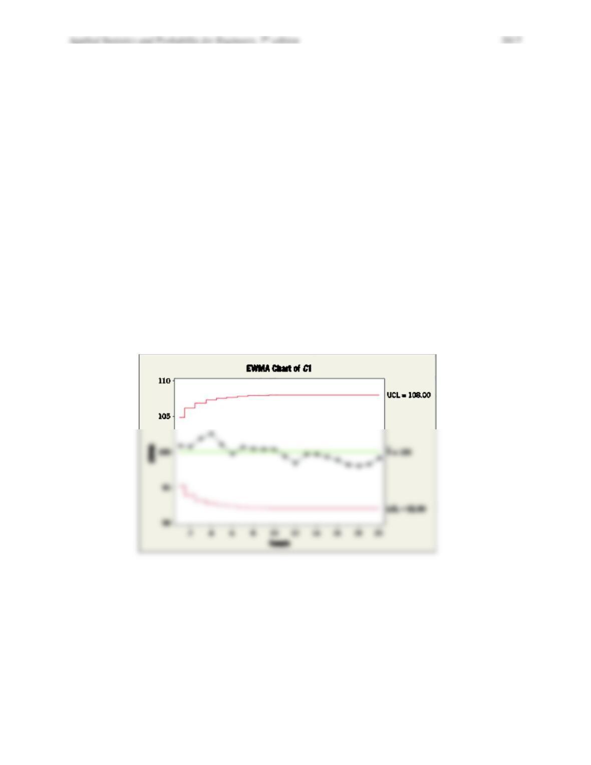
(a) Construct an EWMA control chart with
= 0.2. Does the process appear to be in control?
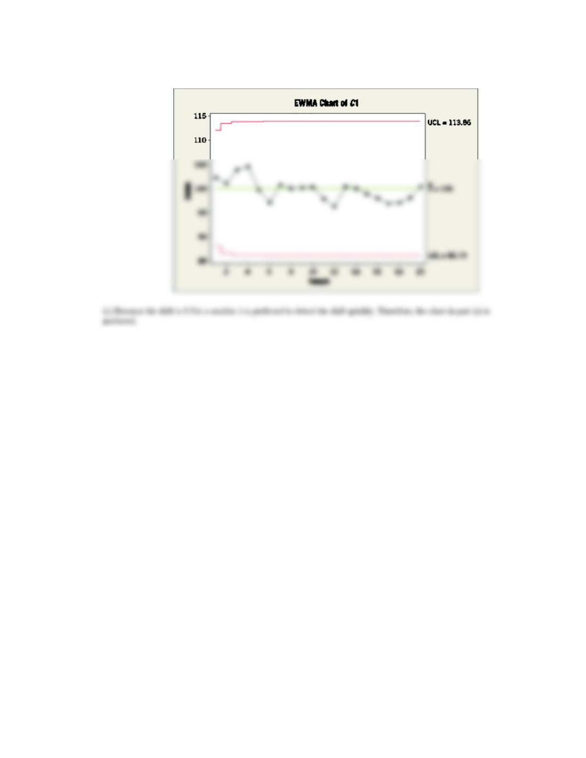
(b) Construct an EWMA control chart with
= 0.5. Compare your results to part (a).
(c) If the concentration shifted to 104, would you prefer the chart in part (a) or (b)? Explain.
(a) The process appears to be in control.
Applied Statistics and Probability for Engineers, 7th edition 2017
15–42
(b) The process appears to be in control.
15.8.5 Heart rate (in counts/minute) is measured every 30 minutes. The results of 20 consecutive measurements are as follows:
Use μ = 70 and σ = 3.
Sample
Heart Rate
Sample
Heart Rate
1
68
11
79
2
71
12
79
3
67
13
78
4
69
14
78
5
71
15
78
6
70
16
79
7
69
17
79
8
67
18
82
9
70
19
82
10
70
20
81
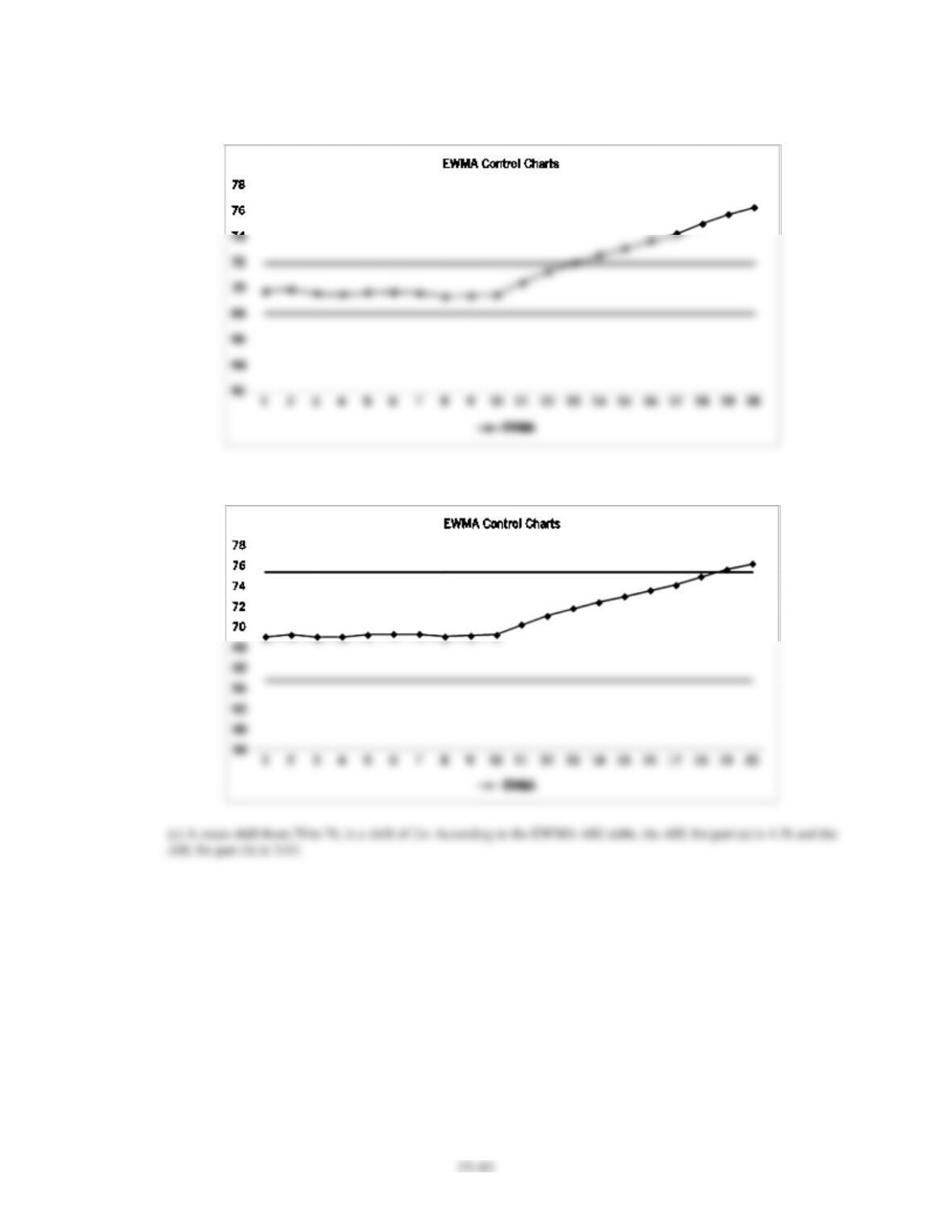
(a) Construct an EWMA control chart with
= 0.1. Use L = 2.81. Does the process appear to be in control?
(b) Construct an EWMA control chart with
= 0.5. Use L = 3.07. Compare your results to those in part (a).
(c) If the heart rate mean shifts to 76, approximate the ARLs for the charts in parts (a) and (b).
Applied Statistics and Probability for Engineers, 7th edition 2017
(a) UCL = 71.93 and LCL = 68.07, the chart signals at observation 13.
(b) UCL = 75.32 and LCL = 64.68, the chart signals at observation 19.
15–44
15.8.6 The number of influenza patients (in thousands) visiting hospitals weekly is shown in the following table.
Use μ = 160 and σ = 2.
Sample
Number of Patients
Sample
Number of Patients
1
162.27
13
159.989
2
157.47
14
159.09
3
157.065
15
162.699
4
160.45
16
163.89
5
157.993
17
164.247
6
162.27
18
162.7
7
160.652
19
164.859
8
159.09
20
163.65
9
157.442
21
165.99
10
160.78
22
163.22
11
159.138
23
164.338
12
161.08
24
164.83
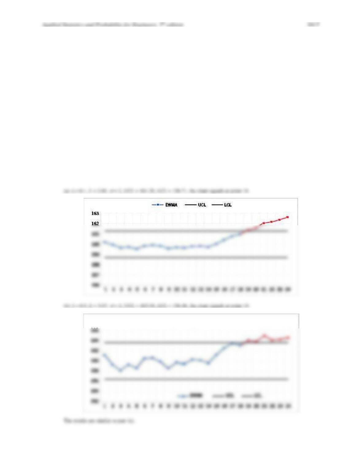
(a) Construct an EWMA control chart with
= 0.1. Use L = 2.81. Does the process appear to be in control?
(b) Construct an EWMA control chart with
= 0.5. Use L = 3.07. Compare your results to those in part (a).
Applied Statistics and Probability for Engineers, 7th edition 2017
Section 15-10
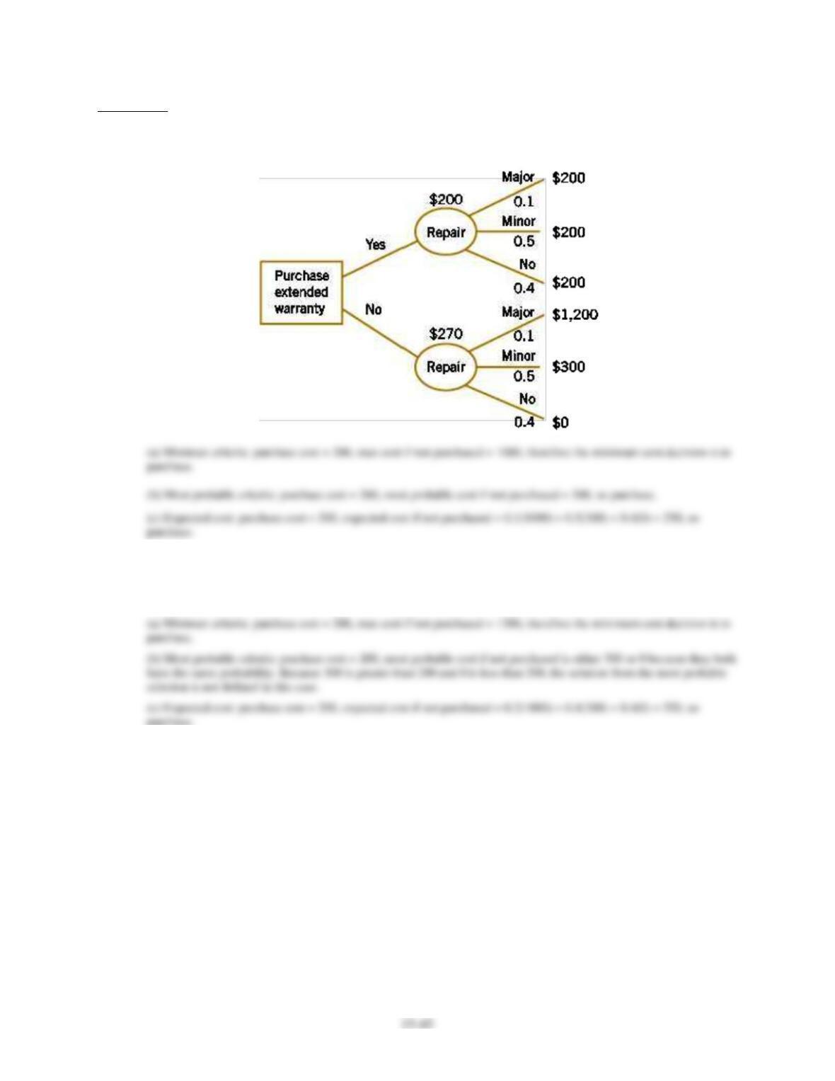
15.10.1 Suppose that the cost of a major repair without the extended warranty in Example 15-8 is changed to $1000.
Determine the decision selected based on the minimax, most probable, and expected cost criteria.
15.10.2 Reconsider the extended warranty decision in Example 15-8. Suppose that the probabilities of the major, minor,
and no repair states are changed to 0.2, 0.4, and 0.4, respectively. Determine the decision selected based on the
minimax, most probable, and expected cost criteria.
15–46
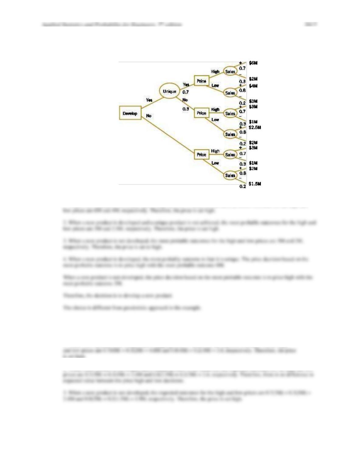
15.10.3 Analyze Example 15-9 based on the most probable criterion and determine the actions that are selected at each decision
node. Do any actions differ from those selected in the example?
Decisions:
1. When a new product is developed and a unique product is achieved, the most probable outcomes for the high and
15.10.4 Analyze Example 15-9 based on the expected profit criterion and determine the actions that are selected at each
decision node. Do any actions differ from those selected in the example?
Decisions:
1. When a new product is developed and a unique product is achieved, the expected outcomes for the high
2. When a new product is developed and a unique product is not achieved, the expected outcomes for the high and low

Applied Statistics and Probability for Engineers, 7th edition 2017
15–47
Supplementary Exercises
15.S7 The diameter of fuse pins used in an aircraft engine application is an important quality characteristic. Twenty-five
samples of three pins each are shown as follows:
Sample Number
Diameter
1
64.030
64.002
64.019
2
63.995
63.992
64.001
3
63.988
64.024
64.021
4
64.002
63.996
63.993
5
63.992
64.007
64.015
6
64.009
63.994
63.997
7
63.995
64.006
63.994
8
63.985
64.003
63.993
9
64.008
63.995
64.009
10
63.998
74.000
63.990
11
63.994
63.998
63.994
12
64.004
64.000
64.007
13
63.983
64.002
63.998
14
64.006
63.967
63.994
15
64.012
64.014
63.998
16
64.000
63.984
64.005
17
63.994
64.012
63.986
18
64.006
64.010
64.018
19
63.984
64.002
64.003
20
64.000
64.010
64.013
21
63.988
64.001
64.009
22
64.004
63.999
63.990
23
64.010
63.989
63.990
24
64.015
64.008
63.993
25
63.982
63.984
63.995
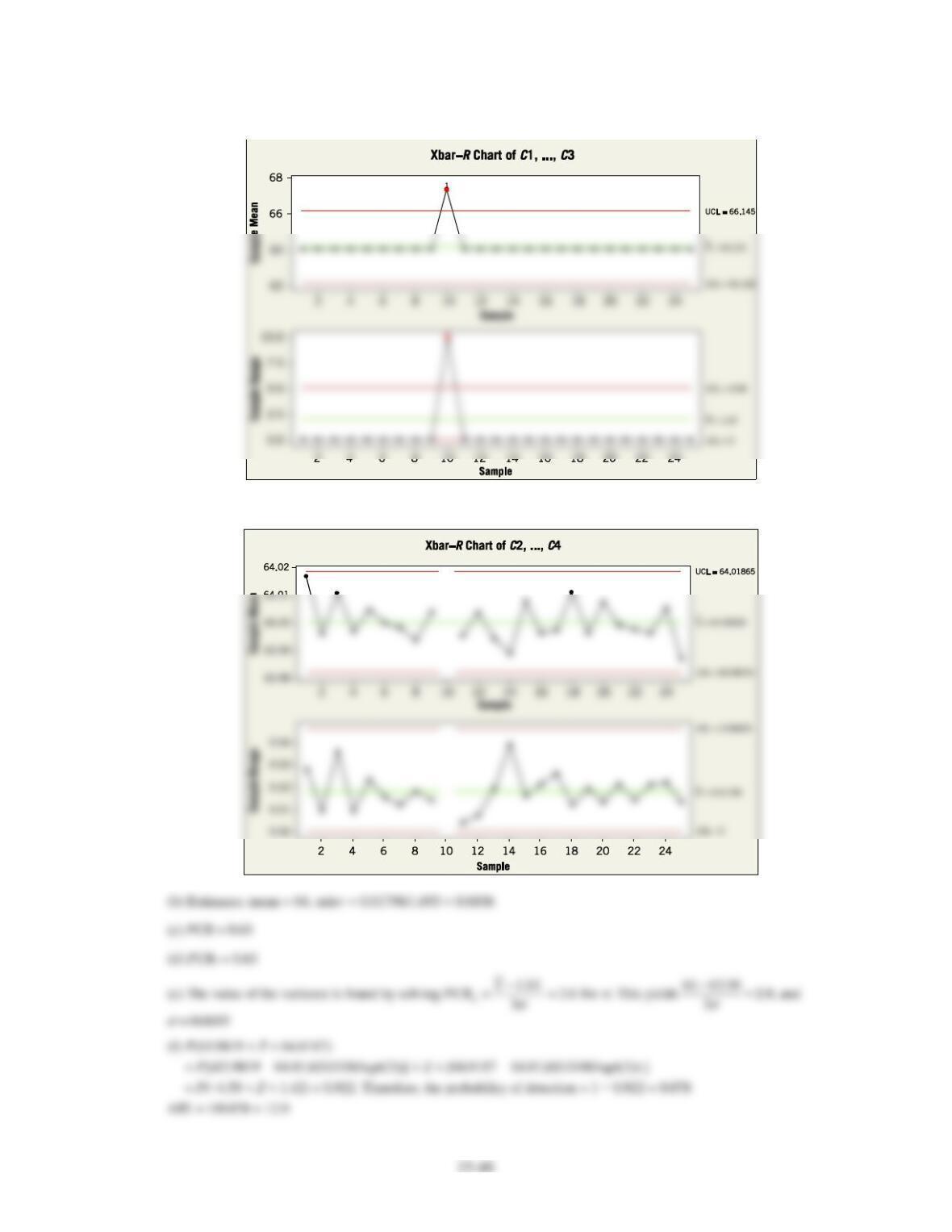
(a) Set up
X
and R charts for this process. If necessary, revise limits so that no observations are out of control.
(b) Estimate the process mean and standard deviation.
(c) Suppose that the process specifications are at 64 ± 0.02. Calculate an estimate of PCR. Does the process meet a
minimum capability level of PCR ≥ 1.33?
(d) Calculate an estimate of PCRk. Use this ratio to draw conclusions about process capability.
(e) To make this process a 6-sigma process, the variance
2 would have to be decreased such that PCRk = 2.0. What
should this new variance value be?
(f) Suppose that the mean shifts to 64.01. What is the probability that this shift is detected on the next sample? What is
the ARL after the shift?
Applied Statistics and Probability for Engineers, 7th edition 2017
(a) The process is not in control. The control chart follows.
Sample 10 is removed to obtain the following chart.
15–49
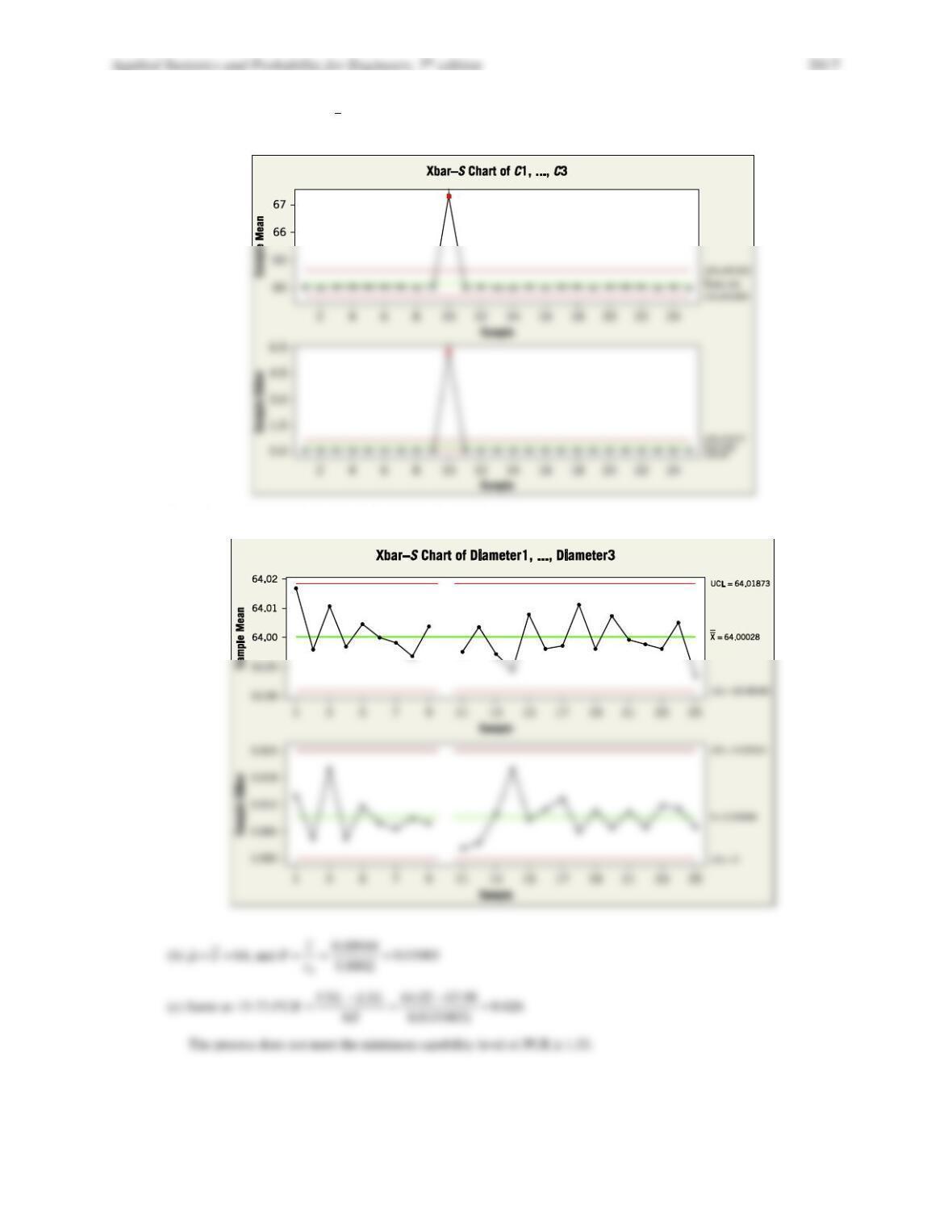
15.S8 Rework Exercise 15.S1 with
X
and S charts.
(a)
The following chart is obtained with subgroup 10 excluded:
Applied Statistics and Probability for Engineers, 7th edition 2017
15–50
(e) Same as the referenced exercise
(f)
− − −
=
63.9818 64.01 64.0187 64.01
(63.98 64.02) 0.01065 / 3 0.01065 / 3
x
X
P X P
15.S9 Plastic bottles for liquid laundry detergent are formed by blow molding. Twenty samples of n = 100 bottles are
inspected in time order of production, and the fraction defective in each sample is reported. The data are as follows:
Sample
Fraction Defective
1
0.12
2
0.15
3
0.18
4
0.10
5
0.12
6
0.11
7
0.05
8
0.09
9
0.13
10
0.13
11
0.10
12
0.07
13
0.12
14
0.08
15
0.09
16
0.15
17
0.10
18
0.06
19
0.12
20
0.13
(a) Set up a P chart for this process. Is the process in statistical control?
Applied Statistics and Probability for Engineers, 7th edition 2017
15–51
(b) Suppose that instead of n = 100, n = 200. Use the data given to set up a P chart for this process. Revise the control
limits if necessary.
(c) Compare your control limits for the P charts in parts (a) and (b) Explain why they differ. Also, explain why your
assessment about statistical control differs for the two sizes of n.
(a)
(b)
Applied Statistics and Probability for Engineers, 7th edition 2017
15–52
15.S10 The following data from the U.S. Department of Energy Web site (www.eia.doe.gov) reported the total U.S. renewable
energy consumption by year (trillion BTU) from 1973 to 2015.
(a) Using all the data, find calculate control limits for a control chart for individual measurements, construct the chart,
and plot the data.
(b) Do the data appear to be generated from an in-control process? Comment on any patterns on the chart.
(a) A control chart for individuals
A control chart for moving ranges
(b) The data does not appear to be generated from an in-control process. Observations at the year 1973–1981, 2001,
Applied Statistics and Probability for Engineers, 7th edition 2017
15–53
15.S11 An article in Quality Engineering [“Is the Process Capable? Tables and Graphs in Assessing Cpm” (1992,
Vol. 4(4)]. Considered manufacturing data. Specifications for the outer diameter of the hubs were 60.3265 ± 0.001 mm.
A random sample of 20 hubs was taken and the data are shown in the following table:
Sample
x
Sample
x
1
60.3262
11
60.3262
2
60.3262
12
60.3262
3
60.3262
13
60.3269
4
60.3266
14
60.3261
5
60.3263
15
60.3265
6
60.3260
16
60.3266
7
60.3262
17
60.3265
8
60.3267
18
60.3268
9
60.3263
19
60.3262
10
60.3269
20
60.3266
(a) Construct a control chart for individual measurements. Revise the control limits if necessary.
(b) Compare your chart in part (a) to one that uses only the last (least significant) digit of each diameter as the
measurement. Explain your conclusion.
(c) Estimate μ and
from the moving range of the revised chart and use this value to estimate PCR and PCRk and
interpret these ratios.
(a) Using I-MR chart.
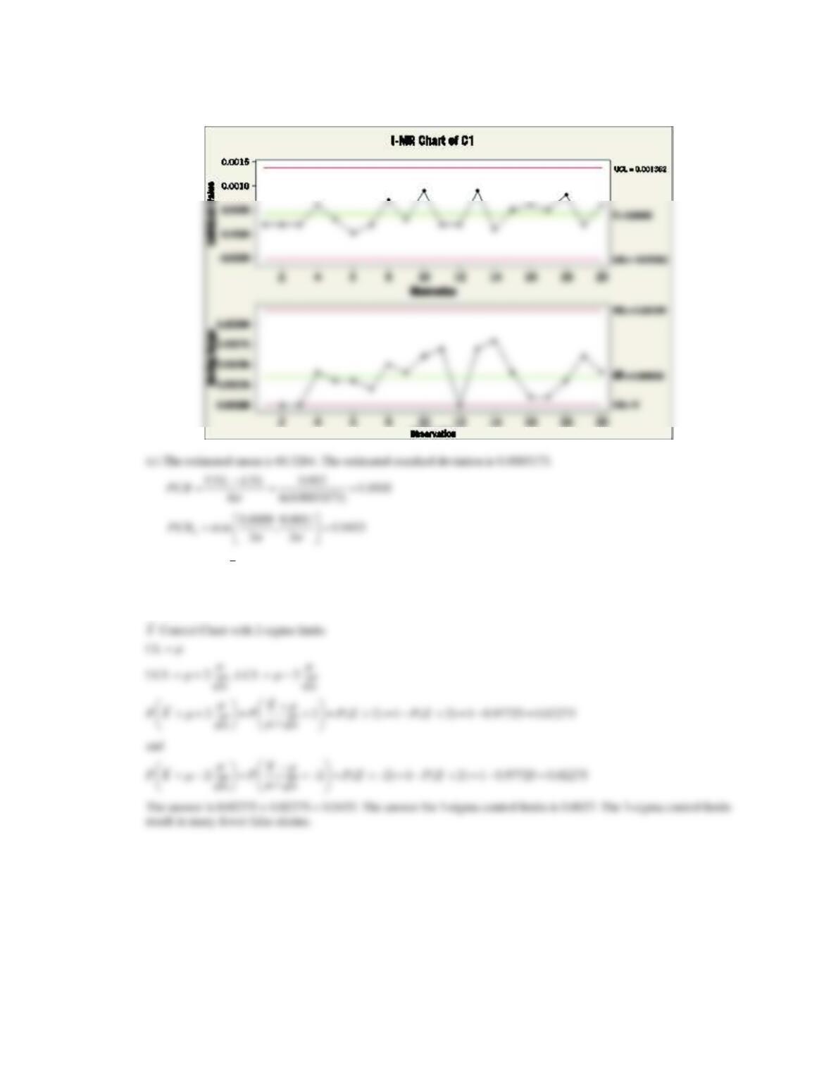
Applied Statistics and Probability for Engineers, 7th edition 2017
15–54
(b) The chart is identical to the chart in part (a) except for the scale of the individuals chart.
15.S12 Suppose that an
X
control chart with 2-sigma limits is used to control a process. Find the probability that a false out-of-
control signal is produced on the next sample. Compare this with the corresponding probability for the chart with 3-
sigma limits and discuss. Comment on when you would prefer to use 2-sigma limits instead of
3-sigma limits.

Applied Statistics and Probability for Engineers, 7th edition 2017
15–55
15.S13 The following dataset was considered in Quality Engineering [“Analytic Examination of Variance Components”
(1994–1995, Vol. 7(2)]. A quality characteristic for cement mortar briquettes was monitored. Samples of size
n = 6 were taken from the process, and 25 samples from the process are shown in the following table:
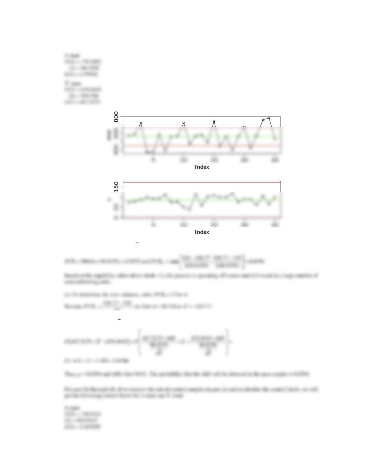
(a) Using all the data, calculate trial control limits for X and S charts. Is the process in control?
Batch
X
s
1
572.00
73.25
2
583.83
79.30
3
720.50
86.44
4
368.67
98.62
5
374.00
92.36
6
580.33
93.50
7
388.33
110.23
8
559.33
74.79
9
562.00
76.53
10
729.00
49.80
11
469.00
40.52
12
566.67
113.82
13
578.33
58.03
14
485.67
103.33
15
746.33
107.88
16
436.33
98.69
17
556.83
99.25
18
390.33
17.35
19
562.33
75.69
20
675.00
90.10
21
416.50
89.27
22
568.33
61.36
23
762.67
105.94
24
786.17
65.05
25
530.67
99.42
(b) Suppose that the specifications are at 580 ± 250. What statements can you make about process capability? Compute
estimates of the appropriate process capability ratios.
(c) To make this process a “6–sigma process,” the variance
2 would have to be decreased such that PCRk = 2.0. What
should this new variance value be?
(d) Suppose the mean shifts to 600. What is the probability that this shift is detected on the next sample? What is the
ARL after the shift?
Applied Statistics and Probability for Engineers, 7th edition 2017
15–56
(a)Trial control limits:
(b) An estimate of
is given by
==
4
/ 86.4208/ 0.9515 90.8259Sc
….
3
(d) The probability that
X
falls within the control limits is
Applied Statistics and Probability for Engineers, 7th edition 2017
15–57
15.S14 Suppose that a process is in control and an
X
chart is used with a sample size of 4 to monitor the process. Suddenly
there is a mean shift of 1.5
.
(a) If 3-sigma control limits are used on the
X
chart, what is the probability that this shift remains undetected for three
consecutive samples?
(b) If 2-sigma control limits are in use on the
X
chart, what is the probability that this shift remains undetected for three
consecutive samples?
(c) Compare your answers to parts (a) and (b) and explain why they differ. Also, which limits you would recommend
using and why?
(a) Let p denote the probability that a point plots outside of the control limits when the mean has shifted from
Applied Statistics and Probability for Engineers, 7th edition 2017
15–58
(b) If 2-sigma control limits were used, then
15.S15 Consider the diameter data in Exercise 15.S1.
(a) Construct an EWMA control chart with
= 0.2 and L = 3. Comment on process control.
(b) Construct an EWMA control chart with
= 0.5 and L = 3 and compare your conclusion to part (a).
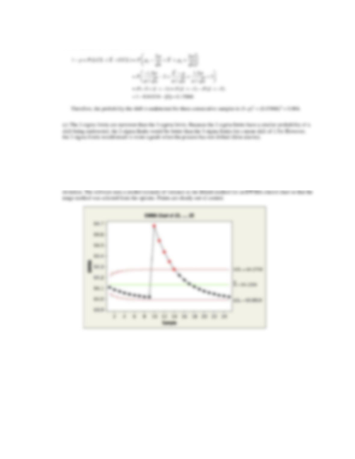
(a) The following control chart use the average range from 25 subgroups of size 3 to estimate the process standard
Applied Statistics and Probability for Engineers, 7th edition 2017
(b) The following control chart use the average range from 25 subgroups of size 3 to estimate the process standard
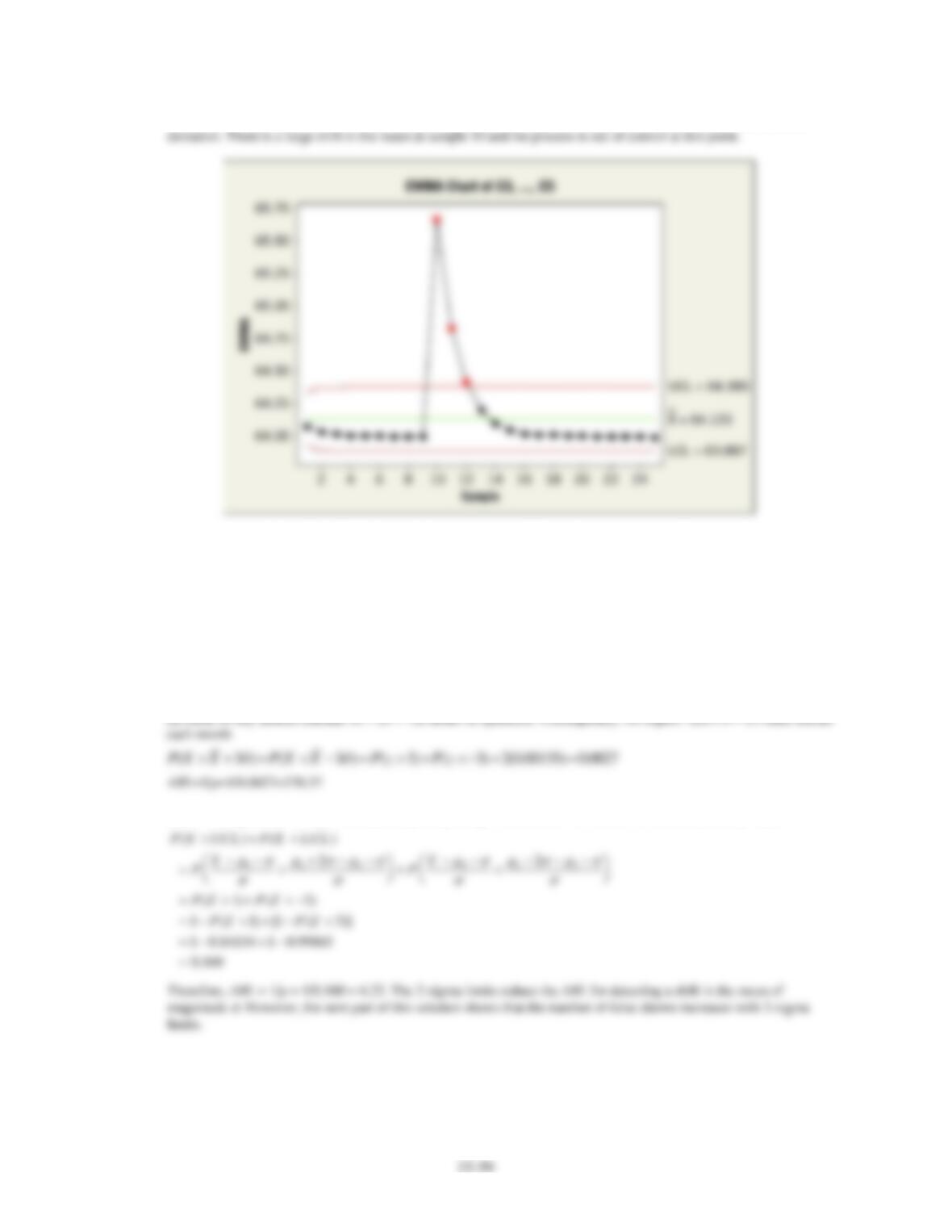
15.S16 Consider a control chart for individuals applied to a continuous 24-hour chemical process with observations taken
every hour.
(a) If the chart has 3-sigma limits, how many false alarms would occur each 30-day month, on the average, with this
chart?
(b) Suppose that the chart has 2-sigma limits. Does this reduce the ARL for detecting a shift in the mean of magnitude
?
(c) Find the in-control ARL if 2-sigma limits are used on the chart. How many false alarms would occur each month
with this chart? Is this in-control ARL performance satisfactory? Explain your answer.
(b) With 2-sigma limits the probability of a point plotting out of control is determined as follows, when μ = μ0 + σ