Dirac Delta Function (5)
Consider the ODE
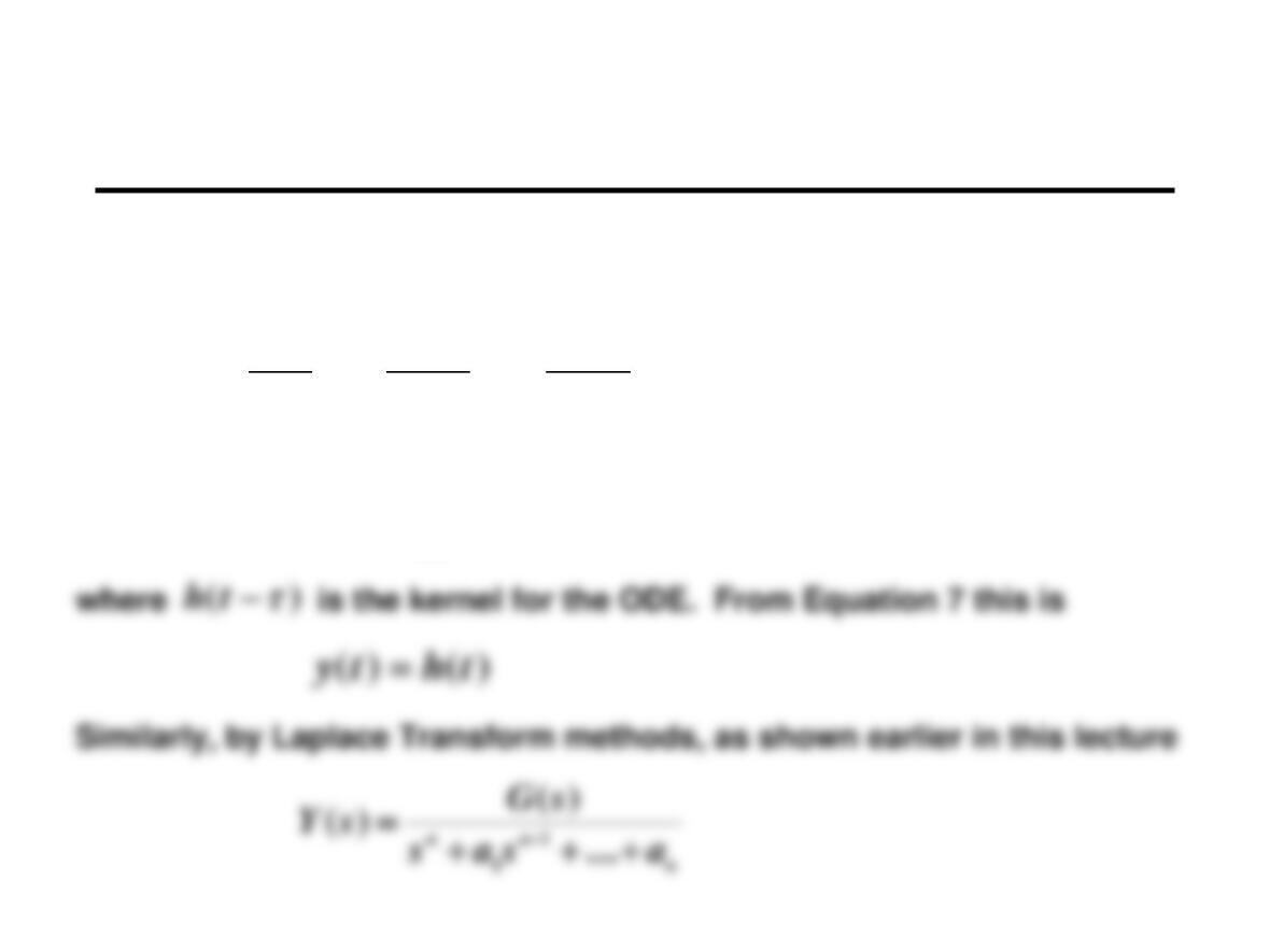
with zero initial conditions. The solution, by time domain methods, is
)(…
2
2
2
1
1
1tya
dt
yd
a
dt
yd
a
dt
yd
n
n
n
n
n
n
n
=++++ −
−
−
−
−= tdthty 0)()()(
Dirac Delta Function (6)
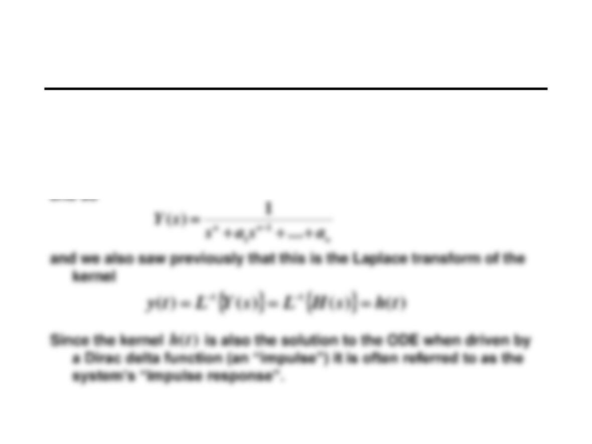
From Equation 8:
1)()( == tLsG
Laplace Transforms
Response to a
(non-repeated) square wave input
Response to
(non-repeated) square wave input
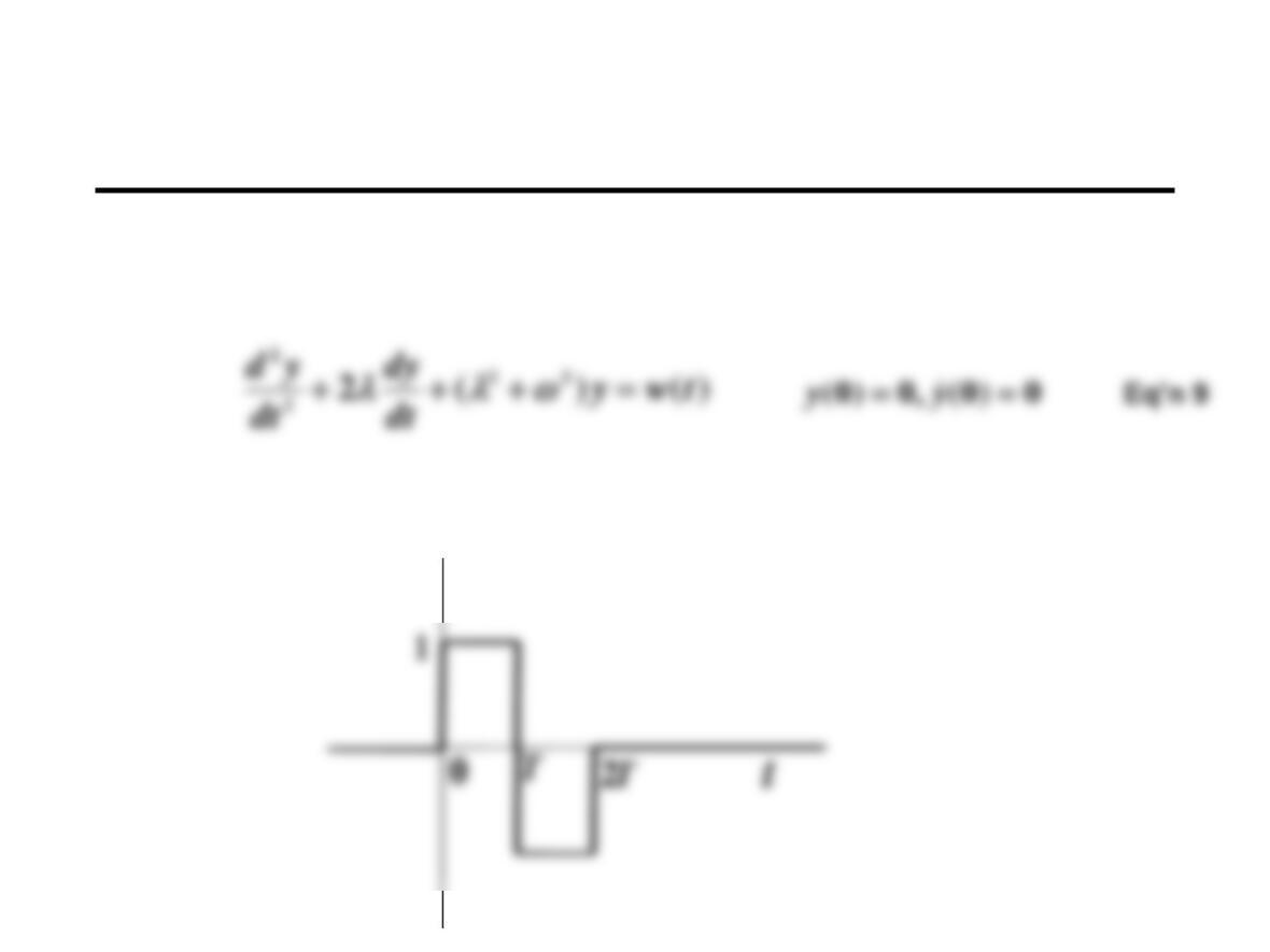
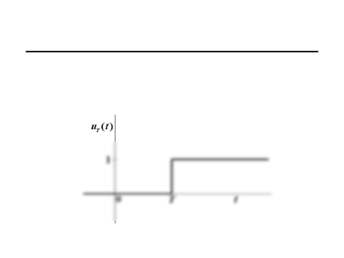
Find the response to
where is a non-repeated square wave beginning at time zero:
)(tw
)(tw
Response to
(non-repeated) square wave input (2)
)(tw
How to describe the input ? It is useful to represent it as a
linear combination of unit step functions:
Response to
(non-repeated) square wave input (3)
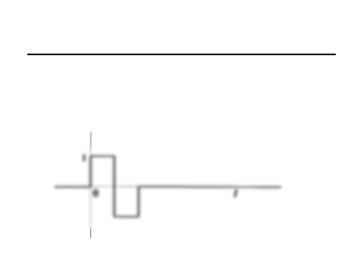
We can describe as composed of several step inputs:
)(tw
)(tw
)()(2)()( 20 tutututw TT +−=
Response to
(non-repeated) square wave input (4)
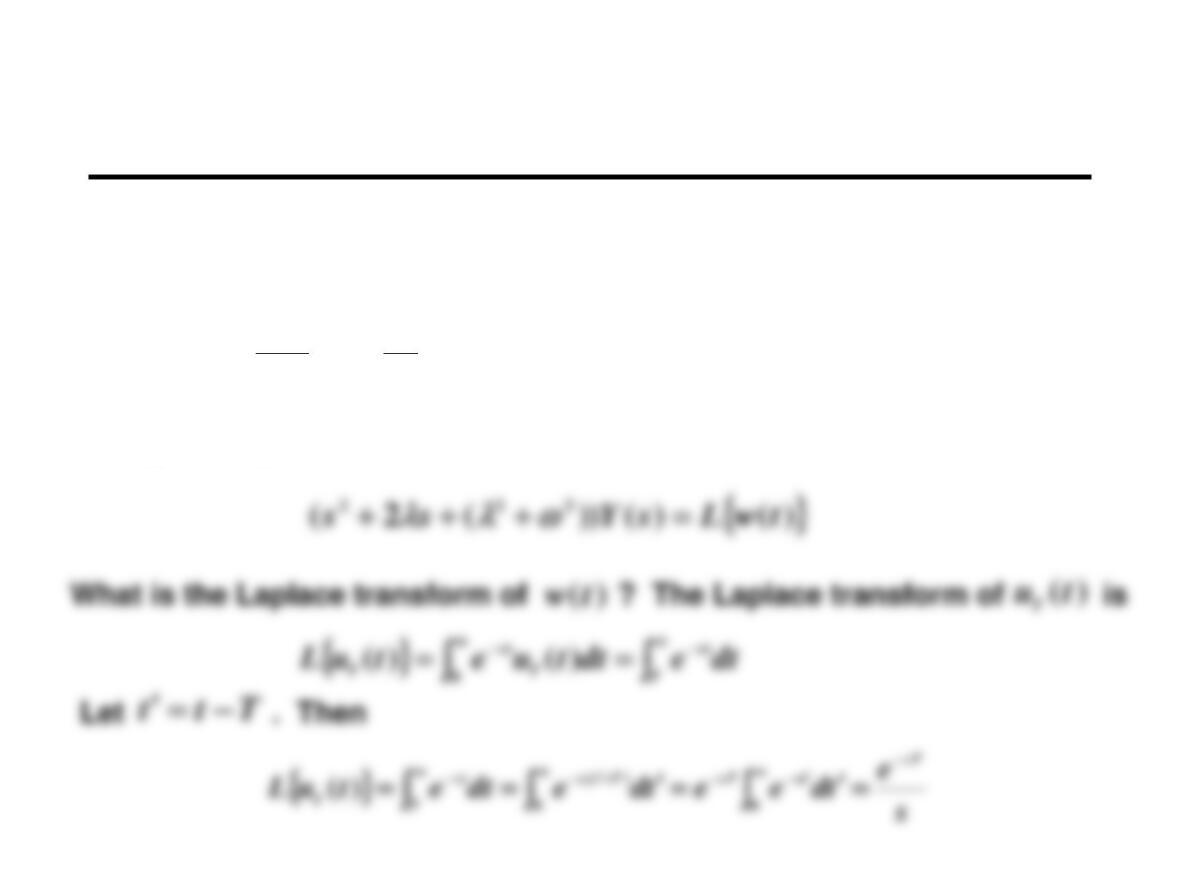
The system equation is then
Taking the Laplace transform of both sides:
)()(2)()(2
20
22
2
2
tututuy
dt
dy
dt
yd
TT
+−=+++
Response to
(non-repeated) square wave input (5)
Solving for :
sTsT eetwLsYss 2222 21)()())(2( −− +−==+++
Therefore
)(sY
Response to
(non-repeated) square wave input (6)
( )
)(2)(2
1
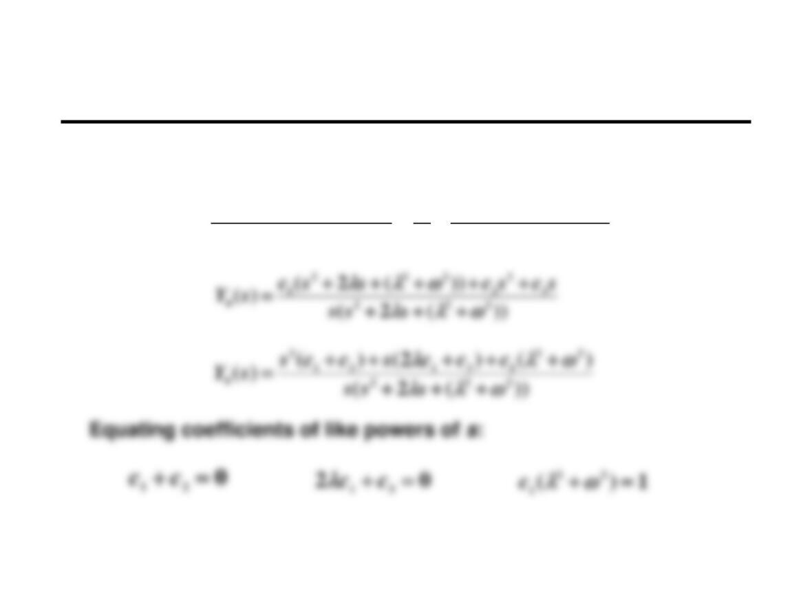
)( 222
321
222
0
+++
+
+=
+++
=ss
csc
s
c
sss
sY
Expanding
)(
0sY
Response to
(non-repeated) square wave input (7)
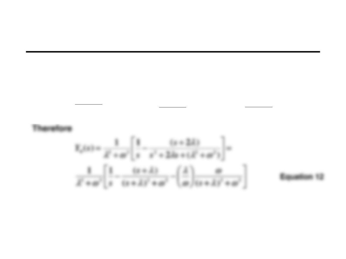
This is three linear equations in three unknowns. The solutions are
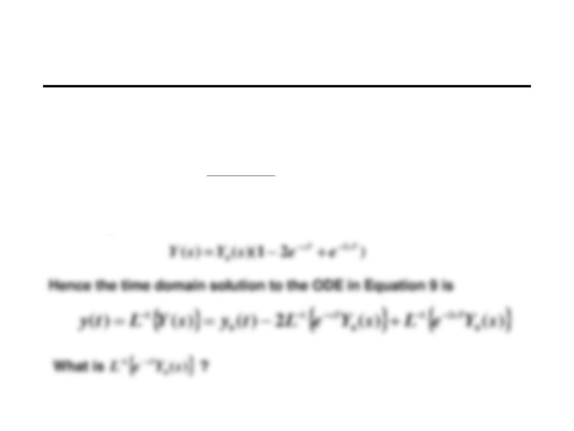
22
1
1
+
=c
22
2
1
+
−
=c
22
3
2
+
−
=c
Response to
(non-repeated) square wave input (8)
Using our short table of Laplace transforms, the time domain
function corresponding to Equation 12 is
)sin)/(cos1(
)(
1
)()( 22
0
1
0tetesYLty tt
−−− −−
+
==
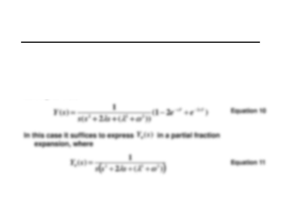
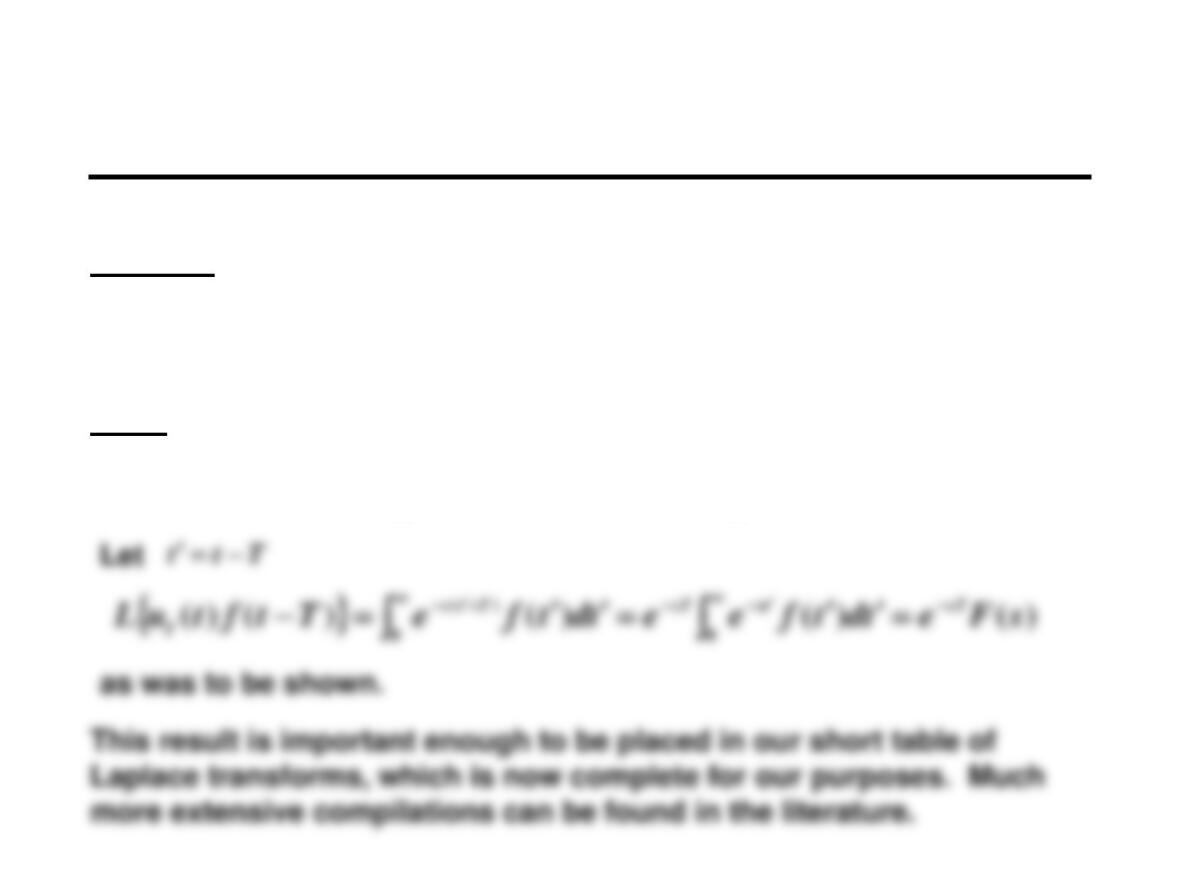
From Equations 10 and 11 we can write
Response to
(non-repeated) square wave input (9)
Theorem:
−
−−=−=− T
st
T
st
TdtTtfedtTtftueTtftuL )()()()()( 0
If is the Laplace transform of a function , then the
Laplace transform of the function delayed by time is
)(sF
)(tf
T
)(sFe sT
−
Proof:
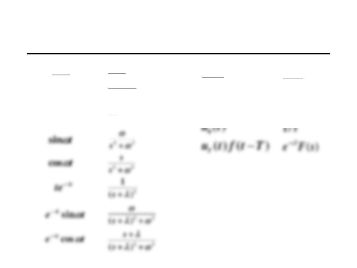
Short Table of Laplace Transforms
2
1
)(
1
)(
+
s
s
sF
)(tf
t
e
−
t
1
)0()(
)(
fssF
sF
−
)(
)(
)(
t
tf
tf