Applied Statistics and Probability for Engineers, 7th edition 2017
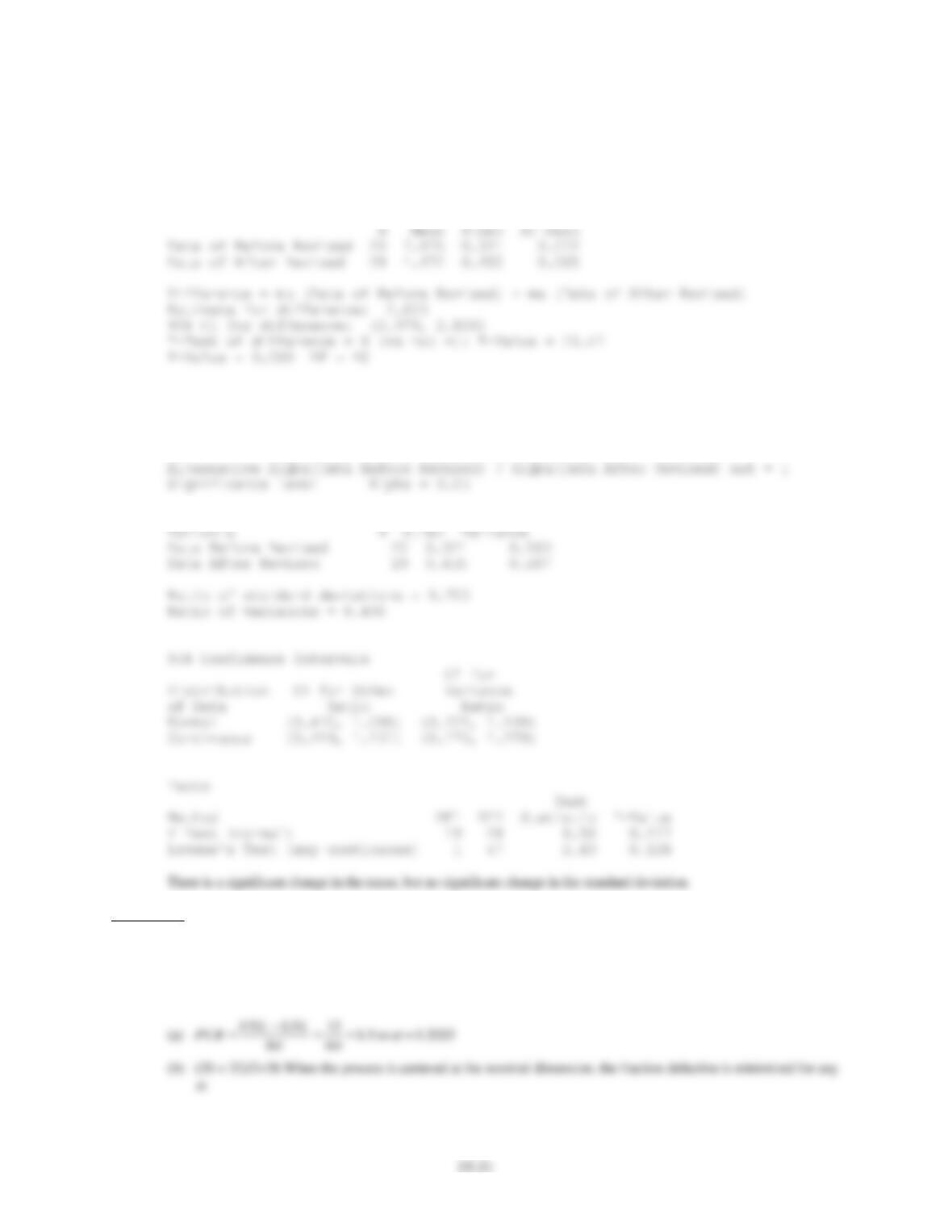
(b) Consider a hypothesis test on the mean and standard deviation of data before and after the change (with point 20
removed from the before dataset and point 19 removed from after dataset)
Hypothesis test on the mean:
Two-sample T for Data Before Revised vs Data After Revised
Hypothesis test on the standard deviation
Method
Null Sigma(Data Before Revised) / Sigma(Data After Revised) = 1
Statistics
Section 15-5
15.5.1 Suppose that a quality characteristic is normally distributed with specifications from 20 to 32 units.
(a) What value is needed for s to achieve a PCR of 1.5?
(b) What value for the process mean minimizes the fraction defective? Does this choice for the mean depend on the
value of
?
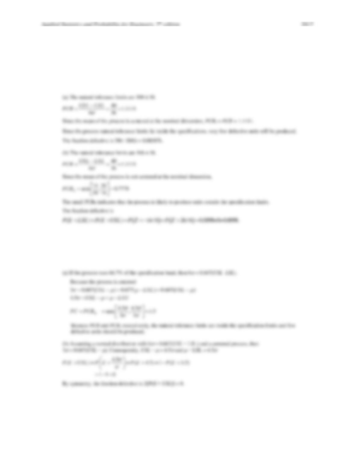
15–22
15.5.2 Suppose that a quality characteristic is normally distributed with specifications at 100 ± 20. The process standard
deviation is 6.
(a) Suppose that the process mean is 100. What are the natural tolerance limits? What is the fraction defective?
Calculate PCR and PCRk and interpret these ratios.
(b) Suppose that the process mean is 106. What are the natural tolerance limits? What is the fraction defective?
Calculate PCR and PCRk and interpret these ratios.
15.5.3 A normally distributed process uses 66.7% of the specification band. It is centered at the nominal dimension, located
halfway between the upper and lower specification limits.
(a) Estimate PCR and PCRk. Interpret these ratios.
(b) What fallout level (fraction defective) is produced?
15.5.4 Reconsider Exercise 15.3.2 in which the specification limits are 14.50 ± 0.50.
(a) What conclusions can you draw about the ability of the process to operate within these limits? Estimate the
percentage of defective items that is produced.
Applied Statistics and Probability for Engineers, 7th edition 2017
15–23
(b) Estimate PCR and PCRk. Interpret these ratios.
(a) Assume a normal distribution with
= 14
ˆ.510
and
= = =
2
0.344
ˆ0.148
2.326
r
d
(b)
−−
= = =
15.00 14.00 1.13
ˆ
6( ) 6(0.148)
USL LS L
PCR
15.5.5 Reconsider Exercise 15.3.1. Suppose that the variable is normally distributed with specifications at 220 ± 50. What is
the proportion out of specifications? Estimate and interpret PCR and PCRk.
(a) Assume a normal distribution with
=
ˆ223
and
= = =
4
13.58
ˆ14.74
0.9213
s
c
( ) ( )
−−
= = = −
=
ˆ170 223 3.60
ˆ14.74
0.00016
LSL
P X LSL P Z P Z P Z
Applied Statistics and Probability for Engineers, 7th edition 2017
15–24
15.5.6 Reconsider the copper-content measurements in Exercise 15.3.6. Given that the specifications are at 6.0 ± 1.0, estimate
PCR and PCRk and interpret these ratios.
Assuming a normal distribution with
=
ˆ6.284
and
== 1.1328
ˆ1.693 0.669
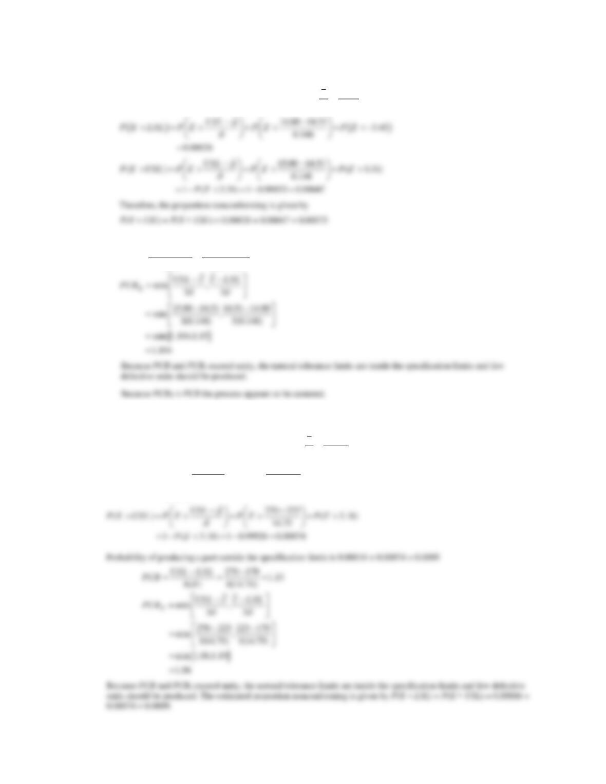
15.5.7 Suppose that a quality characteristic is normally distributed with specifications at 120 ± 20. The process standard
deviation is 6.5.
(a) Suppose that the process mean is 120. What are the natural tolerance limits? What is the fraction defective?
Calculate PCR and PCRk and interpret these ratios.
(b) Suppose that the process mean shifts off-center by 1.5 standard deviations toward the upper specification limit.
Recalculate the quantities in part (a).
(c) Compare the results in parts (a) and (b) and comment on any differences.
(a) The natural tolerance limits are 120 ± 3(6.5) = (100.5, 139.5)
The fraction conforming is
Applied Statistics and Probability for Engineers, 7th edition 2017
15–25
15.5.8 Reconsider the viscosity measurements in Exercise 15.4.2. The specifications are 500 ± 25. Calculate estimates of the
process capability ratios PCR and PCRk for this process and provide an interpretation.
Assuming a normal distribution with
= 5
ˆ00.6
and
= 1
ˆ7.17
−−
= = =
525 475 0.49
USL L SL
PCR
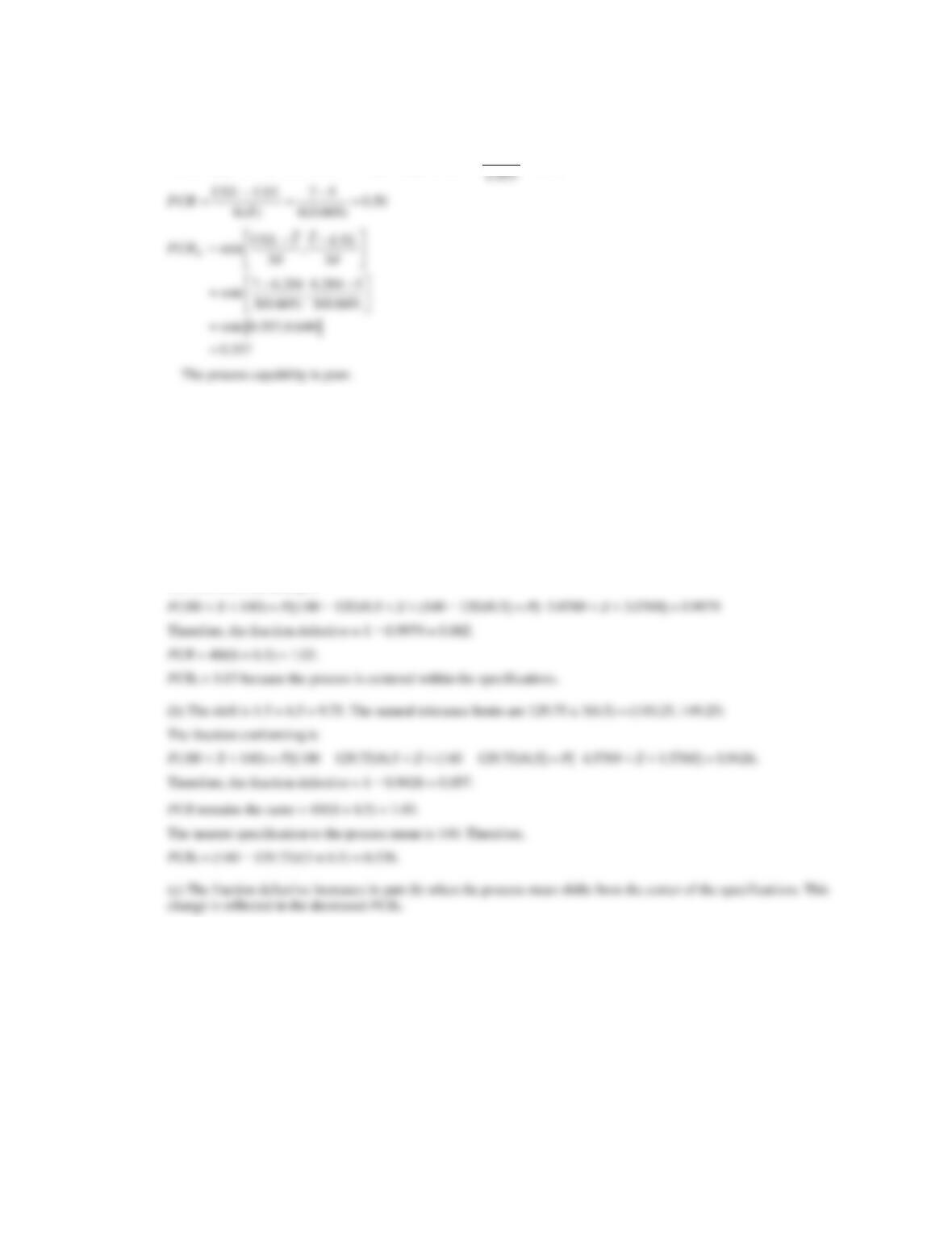
15.5.9 A process mean is centered between the specification limits and PCR = 1.33. Assume that the process mean increases
by 1.5
.
(a) Calculate PCR and PCRk for the shifted process.
(b) Calculate the estimated fallout from the shifted process and compare your result to those in Table 15.4. Assume a
normal distribution for the measurement.
(a) There is no change to
−
==
1.33
6X
USL L S L
PCR
15.5.10 The PCR for a measurement is 1.5 and the control limits for an
X
chart with n = 4 are 24.6 and 32.6.
(a) Estimate the process standard deviation
.
(b) Assume that the specification limits are centered around the process mean. Calculate the specification limits.
−
32.6 24.6 4
Applied Statistics and Probability for Engineers, 7th edition 2017
15–26
Section 15-6
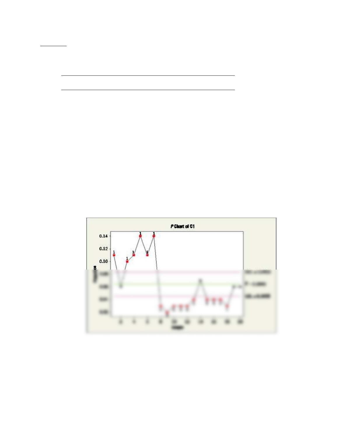
15.6.1 An early example of SPC was described in Industrial Quality Control [“The Introduction of Quality Control at
Colonial Radio Corporation” (1944, Vol. 1(1), pp. 4–9)]. The following are the fractions defective of shaft and washer
assemblies during the month of April in samples of n = 1500 each:
Sample
Fraction Defective
Sample
Fraction
Defective
1
0.11
11
0.03
2
0.06
12
0.03
3
0.1
13
0.04
4
0.11
14
0.07
5
0.14
15
0.04
6
0.11
16
0.04
7
0.14
17
0.04
8
0.03
18
0.03
9
0.02
19
0.06
10
0.03
20
0.06
(a) Set up a P chart for this process. Is this process in statistical control?
(b) Suppose that instead of n = 1500, n = 100. Use the data given to set up a P chart for this process. Revise the control
limits if necessary.
(c) Compare your control limits for the P charts in parts (a) and (b). Explain why they differ. Also, explain why your
assessment about statistical control differs for the two sizes of n.
(a) This process is out of control
Applied Statistics and Probability for Engineers, 7th edition 2017
(b)
The process is still out of control, but not as many points fall outside of the control limits. The control limits are wider
for smaller values of n.
(c) The larger sample size leads to a smaller standard deviation for the proportions and. Thus, narrower control limits.
15–28
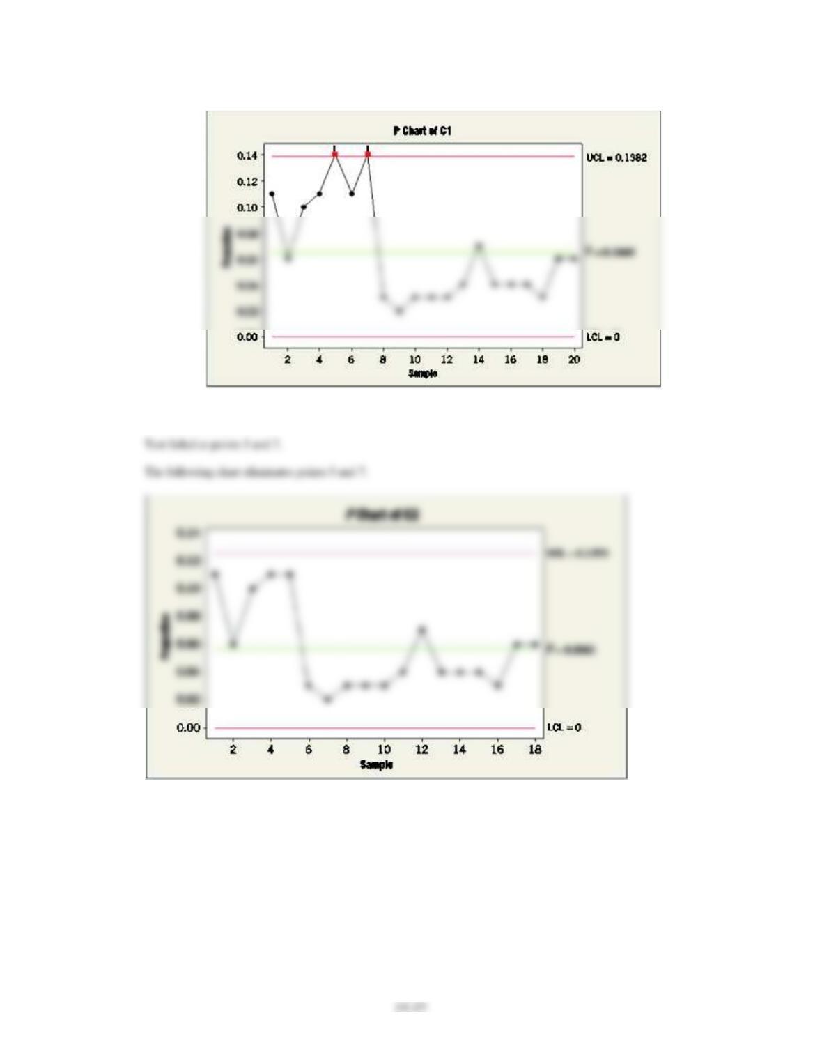
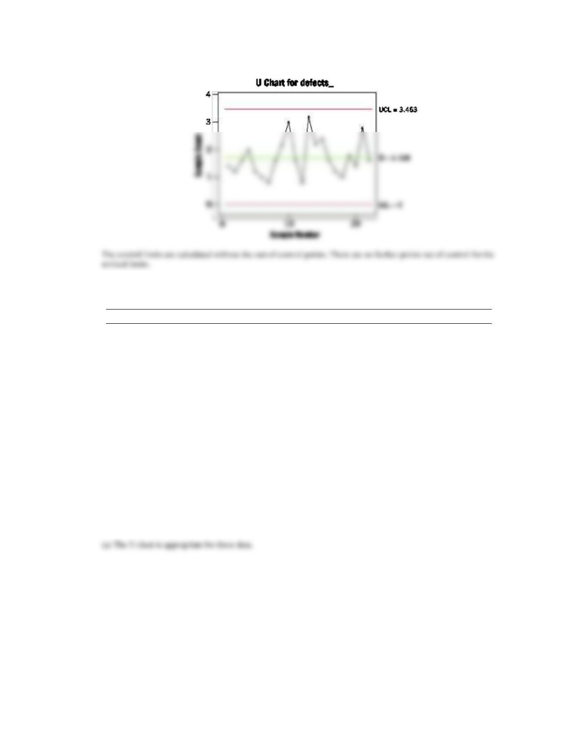
15.6.2 The following represent the number of defects per 1000 feet in rubber-covered wire: 1, 1, 3, 7, 8, 10, 5, 13, 0, 19, 24, 6,
The process does not appear to be in control.
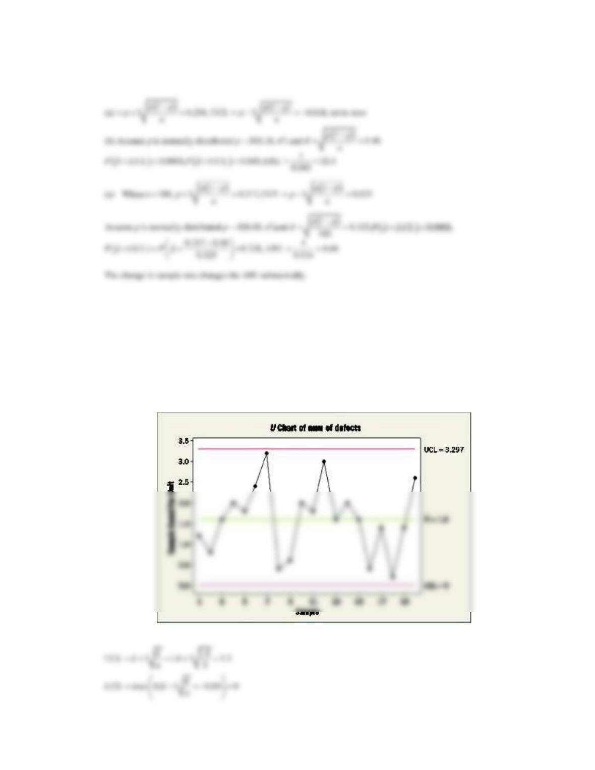
15.6.3 The following represent the number of solder defects observed on 24 samples of five printed circuit boards: 7, 6, 8, 10,
24, 6, 5, 4, 8, 11, 15, 8, 4, 16, 11, 12, 8, 6, 5, 9, 7, 14, 8, 21.
(a) Using all the data, compute trial control limits for a U control chart, construct the chart, and plot the data.
(b) Can we conclude that the process is in control using a U chart? If not, assume that assignable causes can be found,
and list points and revise the control limits.
(a)
Samples 5 and 24 are points beyond the control limits. The limits need to be revised.
Applied Statistics and Probability for Engineers, 7th edition 2017
15–29
(b)
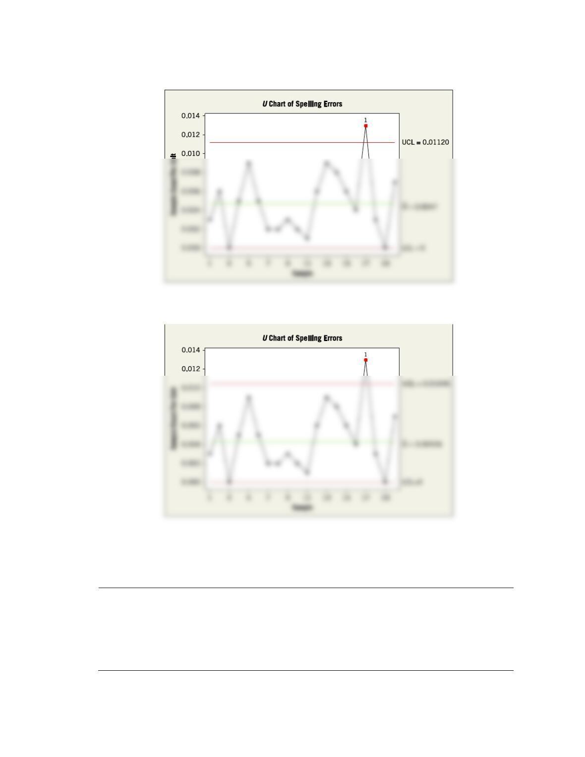
15.6.4 The following data are the number of spelling errors detected for every 1000 words on a news Web site over
20 weeks.
Week
No. of Spelling Errors
Week
No. of Spelling Errors
1
3
11
1
2
6
12
6
3
0
13
9
4
5
14
8
5
9
15
6
6
5
16
4
7
2
17
13
8
2
18
3
9
3
19
0
10
2
20
7
(a) What control chart is most appropriate for these data?
(b) Using all the data, compute trial control limits for the chart in part (a), construct the chart, and plot
the data.
(c) Determine whether the process is in statistical control. If not, assume that assignable causes can be found and out-
of-control points eliminated. Revise the control limits.
Applied Statistics and Probability for Engineers, 7th edition 2017
15–30
(b) The U chart follows.
(c) The process is out-of-control at point 17. The U chart follows with point 17 removed from the calculations for the
control limits.
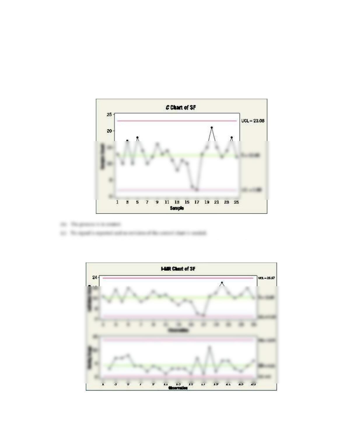
15.6.5 A article of Epilepsy Research [“Statistical Process Control (SPC): A Simple Objective Method for
Monitoring Seizure Frequency and Evaluating Effectiveness of Drug Interventions in Refractory Childhood Epilepsy,”
(2010, Vol. 91, pp. 205–213)] used control charts to monitor weekly seizure changes in patients
with refractory childhood epilepsy. The following table shows representative data of weekly observations of seizure
frequency (SF).
Week
1
2
3
4
5
6
7
8
9
10
SF
13
10
17
10
18
14
10
12
16
13
Week
11
12
13
14
15
16
17
18
19
20
SF
14
11
8
11
10
3
2
13
15
21
Week
21
22
23
24
25
SF
15
12
14
18
12
Applied Statistics and Probability for Engineers, 7th edition 2017
15–31
(a) What type of control chart is appropriate for these data? Construct this chart.
(b) Comment on the control of the process.
(c) If necessary, assume that assignable causes can be found, eliminate suspect points, and revise the control limits.
(d) In the publication, the weekly SFs were approximated as normally distributed and an individual chart was
constructed. Construct this chart and compare it to the attribute chart you built in part (a).
(a) A C-chart is appropriate for these data.
(d) I-chart: UCL = 23.67, CL = 12.48, LCL = 1.29 and both the I-chart and the C-chart indicate that the process is in-
control. The normal approximation to the Poisson distribution becomes reasonable for larger Poisson values.
Applied Statistics and Probability for Engineers, 7th edition 2017
15–32
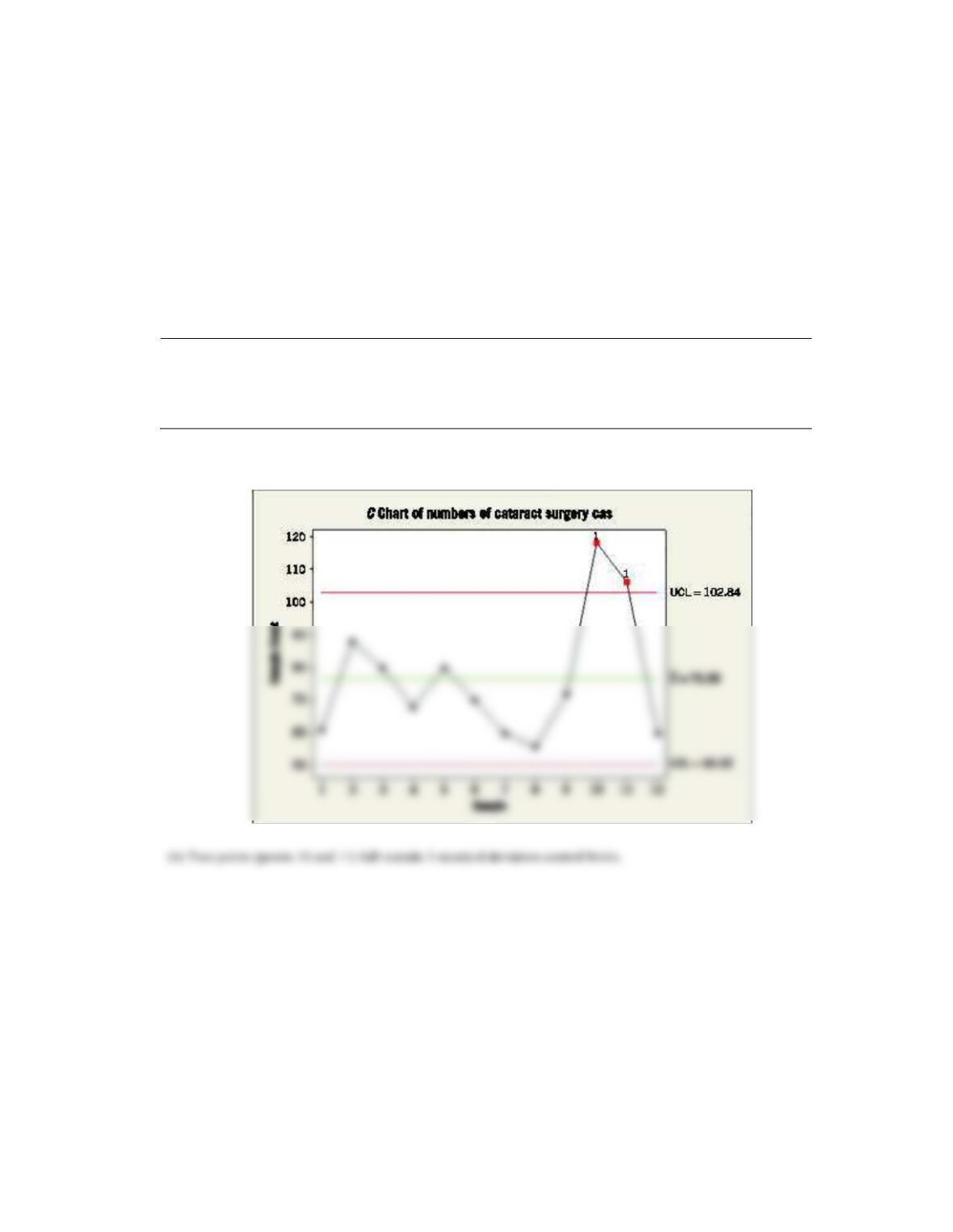
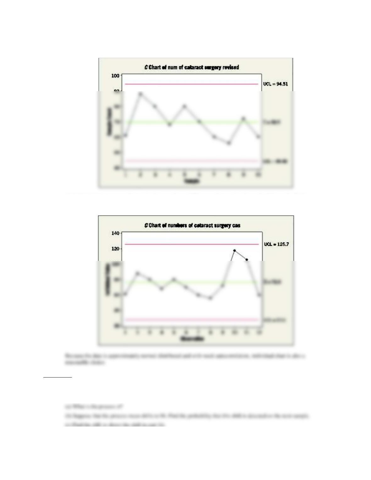
15.6.6 A article in Graefe’s Archive for Clinical and Experimental Ophthalmology [“Statistical Process Control Charts for
Ophthalmology,” (2011, Vol. 249, pp. 1103–1105)] considered the number of cataract surgery cases by month. The
data are shown in the following table.
(a) What type of control chart is appropriate for these data? Construct this chart.
(b) Comment on the control of the process.
(c) If necessary, assume that assignable causes can be found, eliminate suspect points, and revise the control limits.
(d) In the publication, the data were approximated as normally distributed and an individual chart was constructed.
Construct this chart and compare it to the attribute chart you built in part (a). Why might an individual chart be
reasonable?
January
February
March
April
May
June
July
61
88
80
68
80
70
60
August
September
October
November
December
56
72
118
106
60
(a) A C-chart is appropriate for this data.
Applied Statistics and Probability for Engineers, 7th edition 2017
15–33
(c) Assume assignable causes can be found, eliminate these suspect points, and revise the control limits.
(d) Individual chart: no out-of-control points are detected. The normal approximation to the Poisson distribution
becomes reasonable for larger Poisson values.
Section 15-7
15.7.1 An X chart uses samples of size 1. The center line is at 100, and the upper and lower 3-sigma limits are at 112 and
88, respectively.
Applied Statistics and Probability for Engineers, 7th edition 2017
15–34
15.7.2 An
X
chart uses samples of size 4. The center line is at 100, and the upper and lower 3-sigma control limits are at 106
and 94, respectively.
(a) What is the process
?
(b) Suppose that the process mean shifts to 96. Find the probability that this shift is detected on the next sample.
(c) Find the ARL to detect the shift in part (b).
15.7.3 Consider an
X
control chart with UCL = 0.0635, LCL = 0.0624, and n = 5. Suppose that the mean shifts to 0.0625.
(a) What is the probability that this shift is detected on the next sample?
(b) What is the ARL after the shift?
15.7.4 Consider an
X
control chart with UCL = 14.708, LCL = 14.312, and n = 5. Suppose that the mean shifts to 14.6.
Applied Statistics and Probability for Engineers, 7th edition 2017
15–35
(a) What is the probability that this shift is detected on the next sample?
(b) What is the ARL after the shift?
15.7.5 An
X
chart uses a sample of size 3. The center line is at 200, and the upper and lower 3-sigma control limits are
at 212 and 188, respectively. Suppose that the process mean shifts to 195.
(a) Find the probability that this shift is detected on the next sample.
(b) Find the ARL to detect the shift in part (a)
15.7.6 Consider an
X
control chart with UCL = 17.40, LCL = 12.79, and n = 3. Suppose that the mean shifts to 13.
(a) What is the probability that this shift is detected on the next sample?
(b) What is the ARL after the shift?
15.7.7 Consider a P-chart with subgroup size n = 50 and center line at 0.12.
(a) Calculate the LCL and UCL.
(b) Suppose that the true proportion defective changes from 0.12 to 0.18. What is the ARL after the shift? Assume that
the sample proportions are approximately normally distributed.
Applied Statistics and Probability for Engineers, 7th edition 2017
15–36
(c) Rework part (a) and (b) with n = 100 and comment on the difference in ARL. Does the increased sample size change
the ARL substantially?
15.7.8 Consider the U chart for printed circuit boards in Example 15.3.3. The center line = 1.6, UCL = 3.3, and n = 5.
(a) Calculate the LCL and UCL.
(b) Suppose that the true mean defects per unit shifts from 1.6 to 2.4. What is the ARL after the shift? Assume that the
average defects per unit are approximately normally distributed.
(c) Rework part (b) if the true mean defects per unit shifts from 1.6 to 2.0 and comment on the difference
in ARL.
(a)
Applied Statistics and Probability for Engineers, 7th edition 2017
Section 15-8
15.8.1 The following data were considered in Quality Engineering [“Parabolic Control Limits for the Exponentially Weighted
Moving Average Control Charts in Quality Engineering” (1992, Vol. 4(4), pp. 487–495)]. In a chemical plant, the data
for one of the quality characteristics (viscosity) were obtained for each 12-hour batch completion. The results of 15
consecutive measurements are shown in the following table.
Batch
Viscosity
Batch
Viscosity
1
13.3
9
14.6
2
14.5
10
14.1
3
15.3
11
14.3
4
15.3
12
16.1
5
14.3
13
13.1
6
14.8
14
15.5
7
15.2
15
12.6
8
14.9
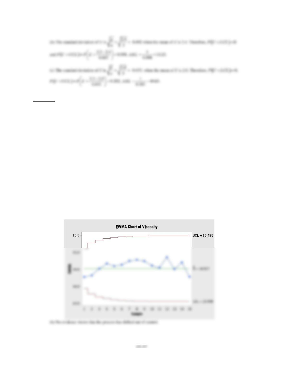
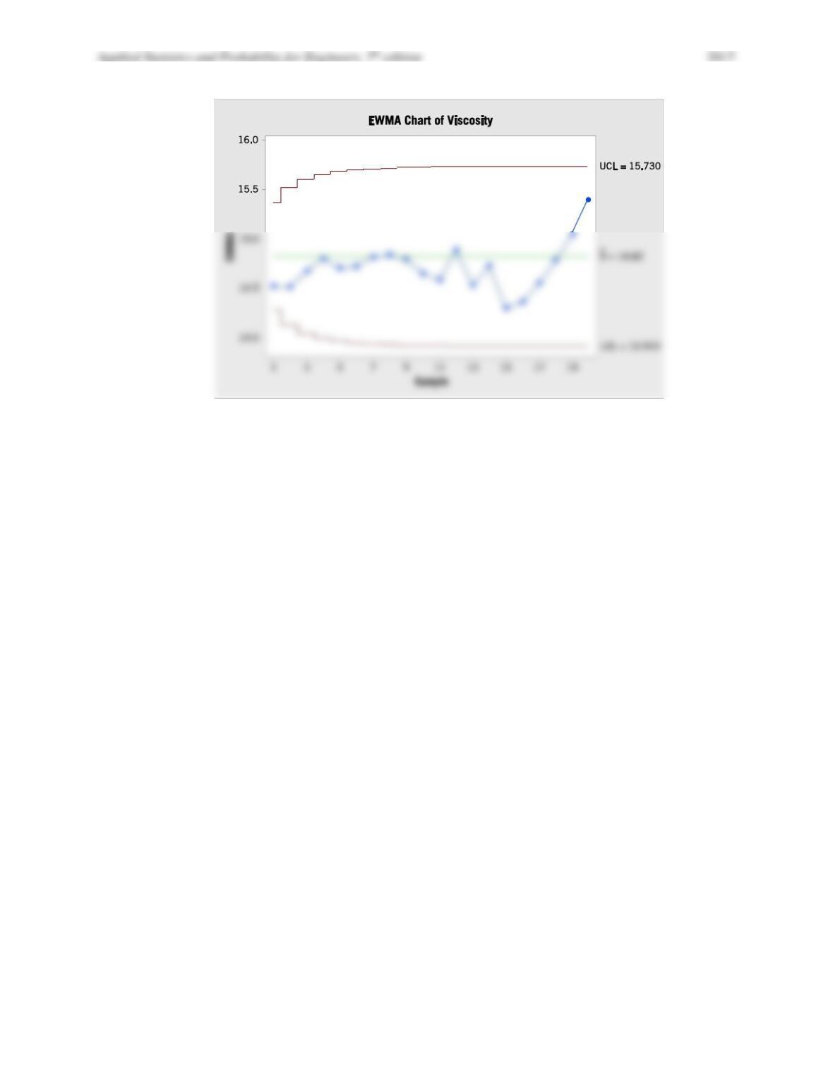
(a) Set up a EWMA control chart for this process with λ = 0.2. Assume that the desired process target is 14.1. Does the
process appear to be in control?
(b)Suppose that the next five observations are 14.6, 15.3, 15.7, 16.1, and 16.8. Apply the EWMA in part (a) to these
new observations. Is there any evidence that the process has shifted out of control?
(a) Yes, this process is in-control. EWMA chart with λ = 0.2 and L = 3 is shown.
15–38
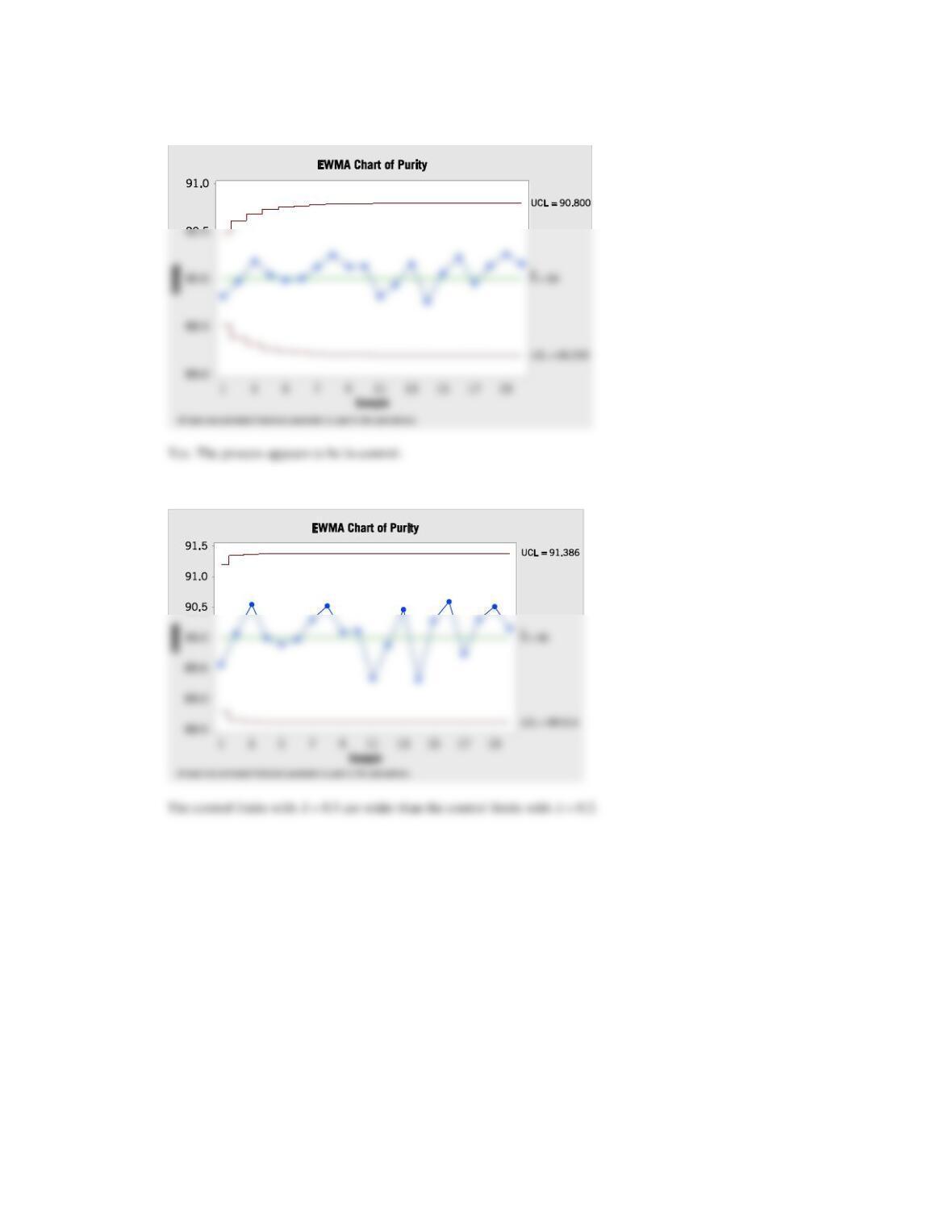
15.8.2 The purity of a chemical product is measured every two hours. The results of 20 consecutive measurements are as
follows:
Sample
Purity
Sample
Purity
1
89.11
11
88.55
2
90.59
12
90.43
3
91.03
13
91.04
4
89.46
14
88.17
5
89.78
15
91.23
6
90.05
16
90.92
7
90.63
17
88.86
8
99.75
18
90.87
9
89.65
19
90.73
10
90.15
20
89.78
Use
= 0.8 and assume that the process target is 90.
(a) Construct an EWMA control chart with
= 0.2. Does the process appear to be in control?
(b) Construct an EWMA control chart with
= 0.5. Compare your results to part (a).
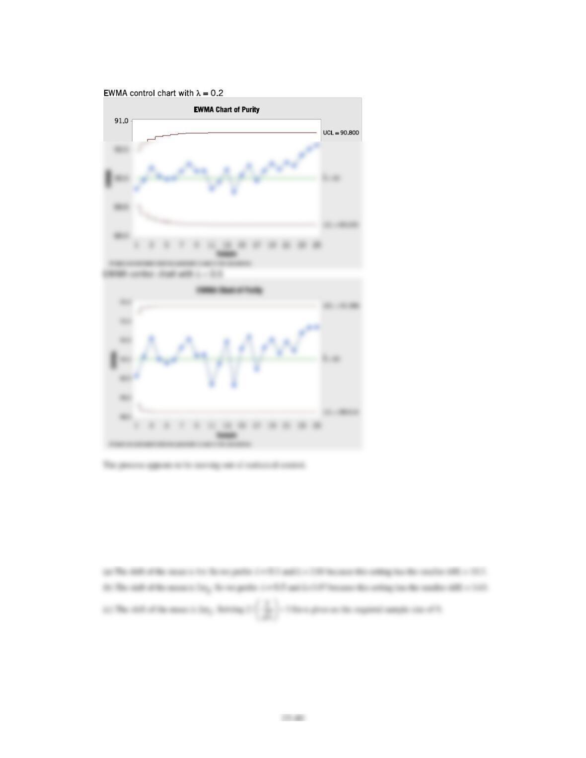
(c) Suppose that the next five observations are 90.75, 90.00, 91.15, 90.95, and 90.86. Apply the EWMAs in parts (a)
and (b) to these new observations. Is there any evidence that the process has shifted out of control
Applied Statistics and Probability for Engineers, 7th edition 2017
15–39
(a)
(b)
Applied Statistics and Probability for Engineers, 7th edition 2017
(c)
15.8.3 Consider an EMWA control chart. The target value for the process is μ0 = 50 and
= 2. Use Table 15.8
(a) If the sample size is n = 1, would you prefer an EWMA chart with
= 0.1 and L = 2.81 or
= 0.5 and
L = 3.07 to detect a shift in the process mean to μ = 52 on average? Why?
(b) If the sample size is increased to n = 4, which chart in part (a) do you prefer? Why?
(c) If an EWMA chart with
= 0.1 and L = 2.81 is used, what sample size is needed to detect a shift to μ = 52 in
approximately three samples on average?