Applied Statistics and Probability for Engineers, 7th edition 2017
15–60
15.S17 Consider the hub data in Exercise 15.S5
(a) Construct an EWMA control chart with
= 0.2 and L = 3. Comment on process control.
(b) Construct an EWMA control chart with
= 0.5 and L = 3 and compare your conclusion to part (a).
(a) The process appears to be in control.
(b) The process appears to be in control.
Applied Statistics and Probability for Engineers, 7th edition 2017
15–61
15.S18 Consider a control chart for individuals with 3-sigma limits. What is the probability that there is not a signal in 3
samples? In 6 samples? In 10 samples?
The probability of having no signal is P(−3 <X< 3) = 0.9973
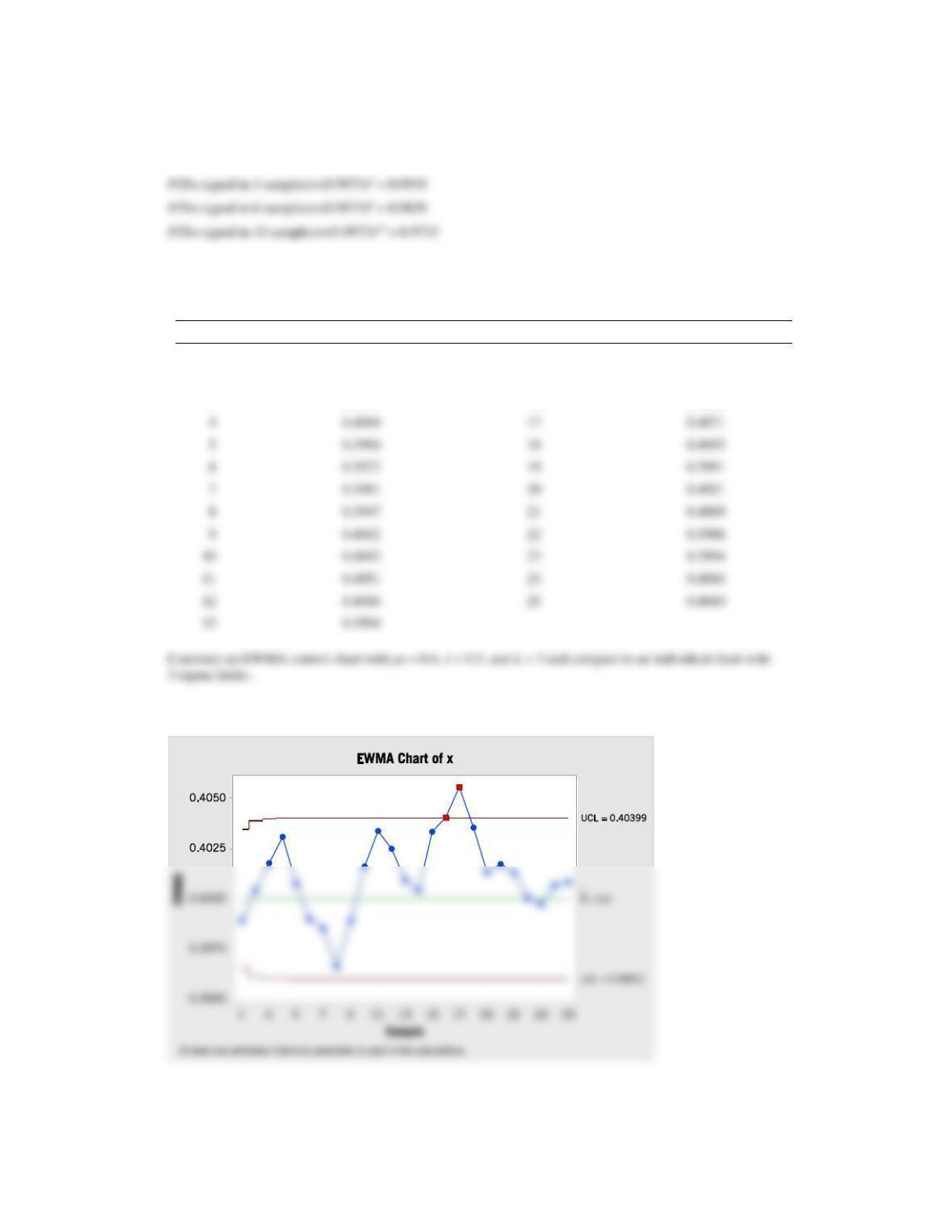
15.S19 The following data were considered in Quality Progress [“Digidot Plots for Process Surveillance” (1990, May, pp. 66–
68)].Measurements of center thickness (in mils) from 25 contact lenses sampled from the production process at regular
intervals are shown in the following table.
Sample
x
Sample
x
1
0.3978
14
0.3999
2
0.4019
15
0.4062
3
0.4031
16
0.4048
4
0.4044
17
0.4071
5
0.3984
18
0.4015
6
0.3972
19
0.3991
7
0.3981
20
0.4021
8
0.3947
21
0.4009
9
0.4012
22
0.3988
0.4043
23
0.3994
0.4051
24
0.4016
0.4016
25
0.4010
0.3994
EWMA control chart
Applied Statistics and Probability for Engineers, 7th edition 2017
15–62
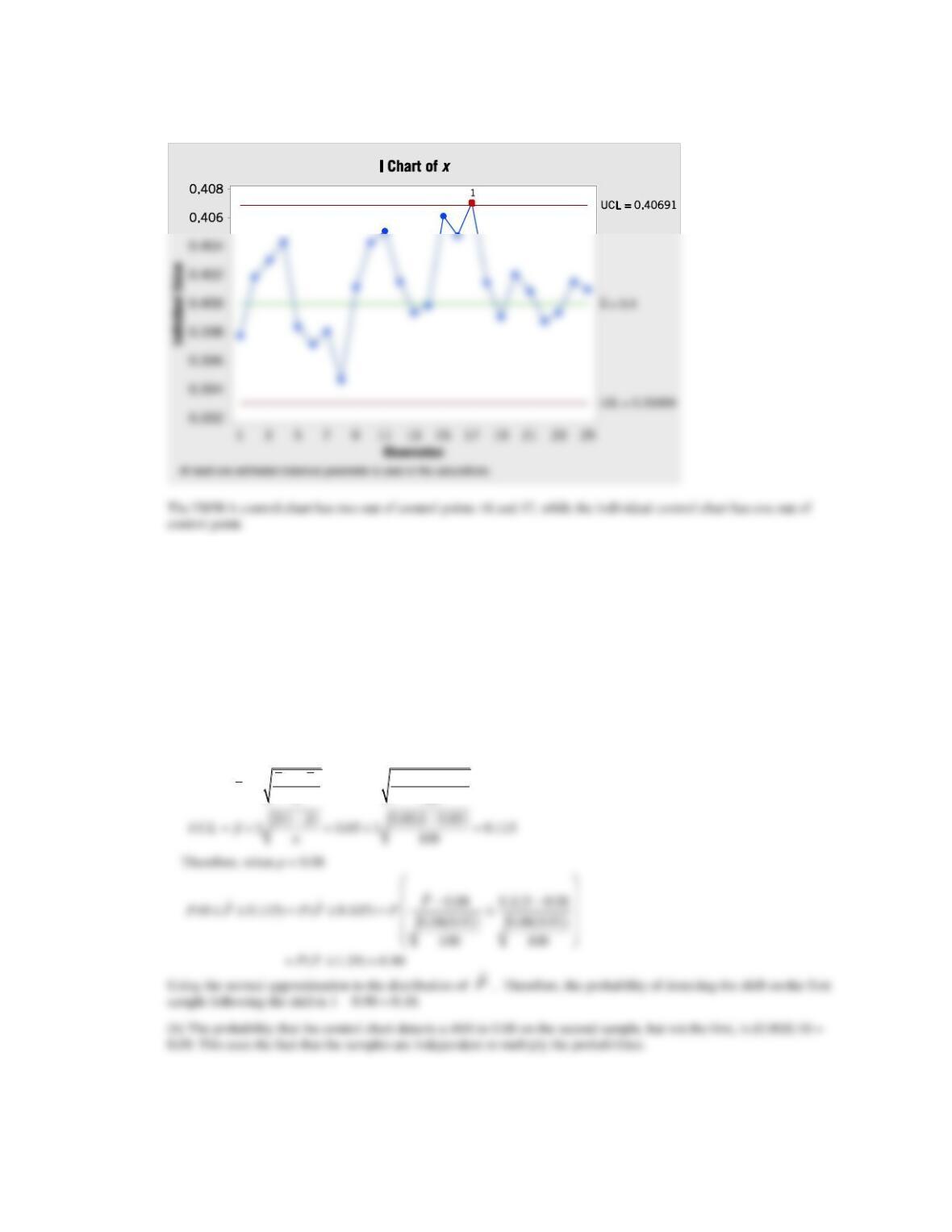
Individual chart with 3 sigma.
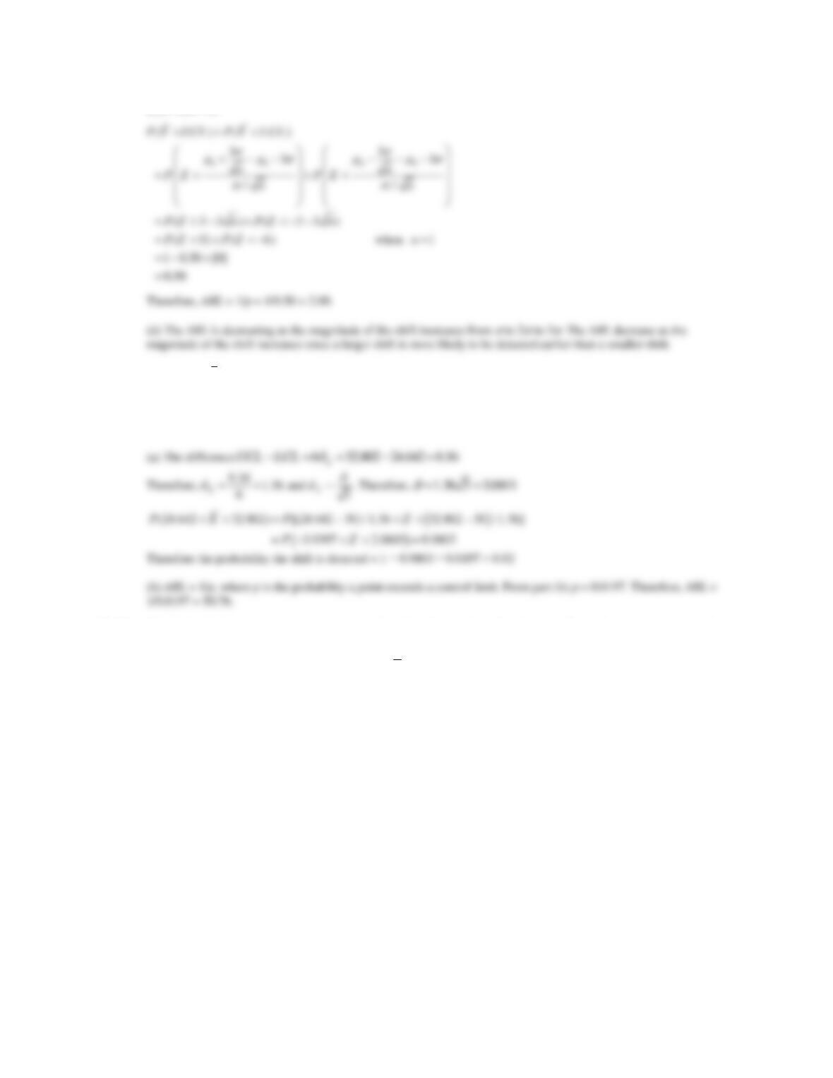
15.S20 A process is controlled by a P chart using samples of size 100. The center line on the chart is 0.05.
(a) What is the probability that the control chart detects a shift to 0.08 on the first sample following the shift?
(b) What is the probability that the control chart does not detect a shift to 0.08 on the first sample following the shift,
but does detect it on the second sample?
(c) Suppose that instead of a shift in the mean to 0.08, the mean shifts to 0.10. Repeat parts (a) and (b).
(d) Compare your answers for a shift to 0.08 and for a shift to 0.10. Explain why they differ. Also, explain why a shift
to 0.10 is easier to detect.
(a) The
ˆ
()P LCL UCLP
, when p = 0.08, is needed.
−−
= − = − = − →
(1 ) 0.05(1 0.05)
3 0.05 3 0.015 0
100
pp
L CL p n
Applied Statistics and Probability for Engineers, 7th edition 2017
15–63
(c) p = 0.10
15.S21 Consider the control chart for individuals with 3-sigma limits.
(a) Suppose that a shift in the process mean of magnitude
occurs. Verify that the ARL for detecting the shift is ARL =
43.9.
(b) Find the ARL for detecting a shift of magnitude 2
in the process mean.
(c) Find the ARL for detecting a shift of magnitude 3
in the process mean.
(d) Compare your responses to parts (a), (b), and (c) and explain why the ARL for detection is decreasing as the
magnitude of the shift increases.
ARL = 1/p where p is the probability a point falls outside the control limits.
(a) μ = μ0 +
and n = 1
(b) μ = μ0+ 2
Applied Statistics and Probability for Engineers, 7th edition 2017
15–64
(c) μ = μ0+ 3
15.S22 Consider an
X
control chart with UCL = 32.802, UCL = 24.642, and n = 5. Suppose that the mean shifts to 30.
(a) What is the probability that this shift is detected on the next sample?
(b) What is the ARL to detect the shift?
15.S23 The depth of a keyway is an important part quality characteristic. Samples of size n = 5 are taken every four hours from
the process, and 20 samples are summarized in the following table.
(a) Using all the data, find trial control limits for
X
and R charts. Is the process in control?
(b) Use the trial control limits from part (a) to identify out-of-control points. If necessary, revise your control limits.
Then estimate the process standard deviation.
(c) Suppose that the specifications are at 140 ± 2. Using the results from part (b), what statements can you make about
process capability? Compute estimates of the appropriate process capability ratios.
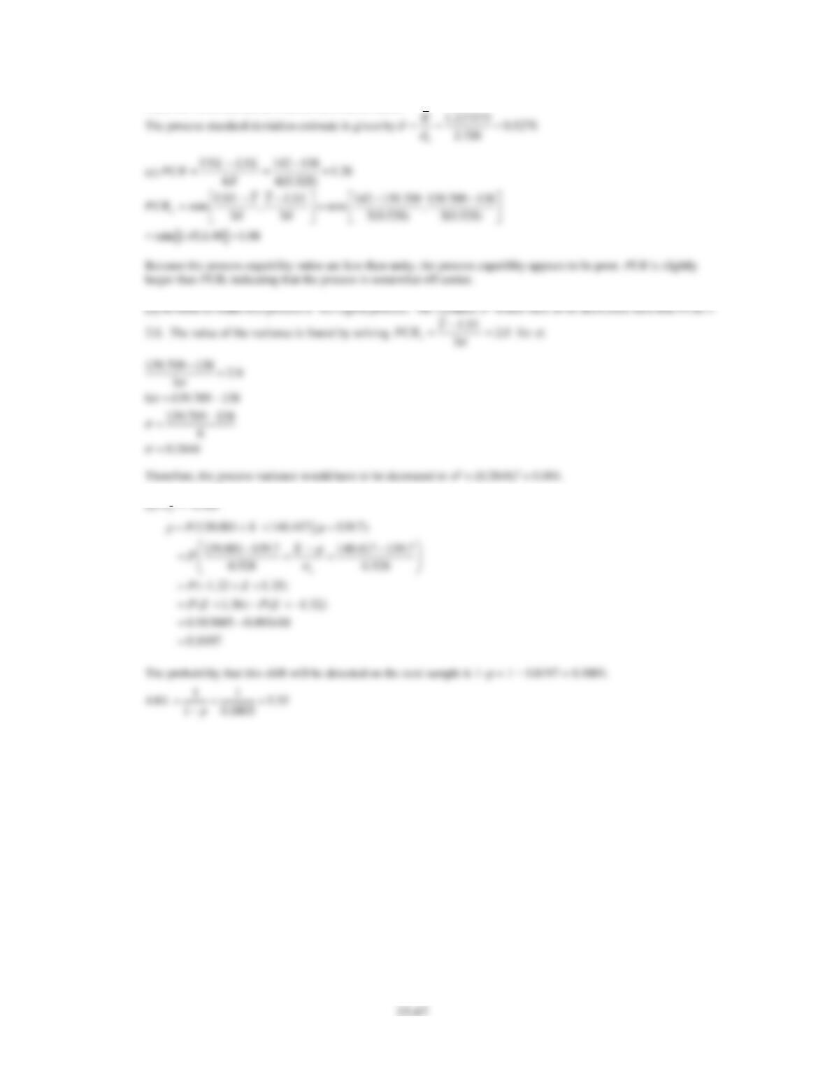
(d) To make this a 6-sigma process, the variance s2 would have to be decreased such that PCRk = 2.0. What should this
new variance value be?

Applied Statistics and Probability for Engineers, 7th edition 2017
15–65
(e) Suppose that the mean shifts to 139.7. What is the probability that this shift is detected on the next sample? What is
the ARL after the shift?
Sample
X
r
1
139.7
1.1
2
139.8
1.4
3
140.0
1.3
4
140.1
1.6
5
139.8
0.9
6
139.9
1.0
7
139.7
1.4
8
140.2
1.2
9
139.3
1.1
10
140.7
1.0
11
138.4
0.8
12
138.5
0.9
13
137.9
1.2
14
138.5
1.1
15
140.8
1.0
16
140.5
1.3
17
139.4
1.4
18
139.9
1.0
19
137.5
1.5
20
139.2
1.3
(a)
X
and Range—Initial Study
Charting
x
X
| Range
Applied Statistics and Probability for Engineers, 7th edition 2017
15–66
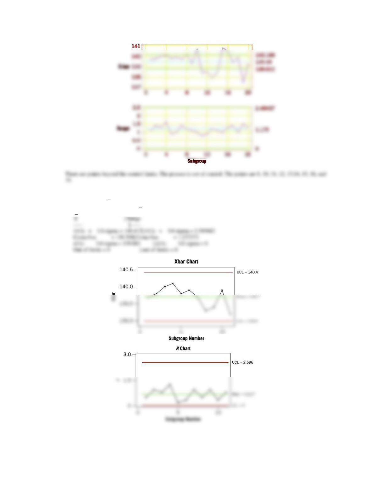
(b) Revised control limits are given in the table below:
X
and Range—Initial Study
Charting
X
X
Applied Statistics and Probability for Engineers, 7th edition 2017
There are no further points beyond the control limits.
2 would have to be decreased such that PCRk =
ˆ.
15–68
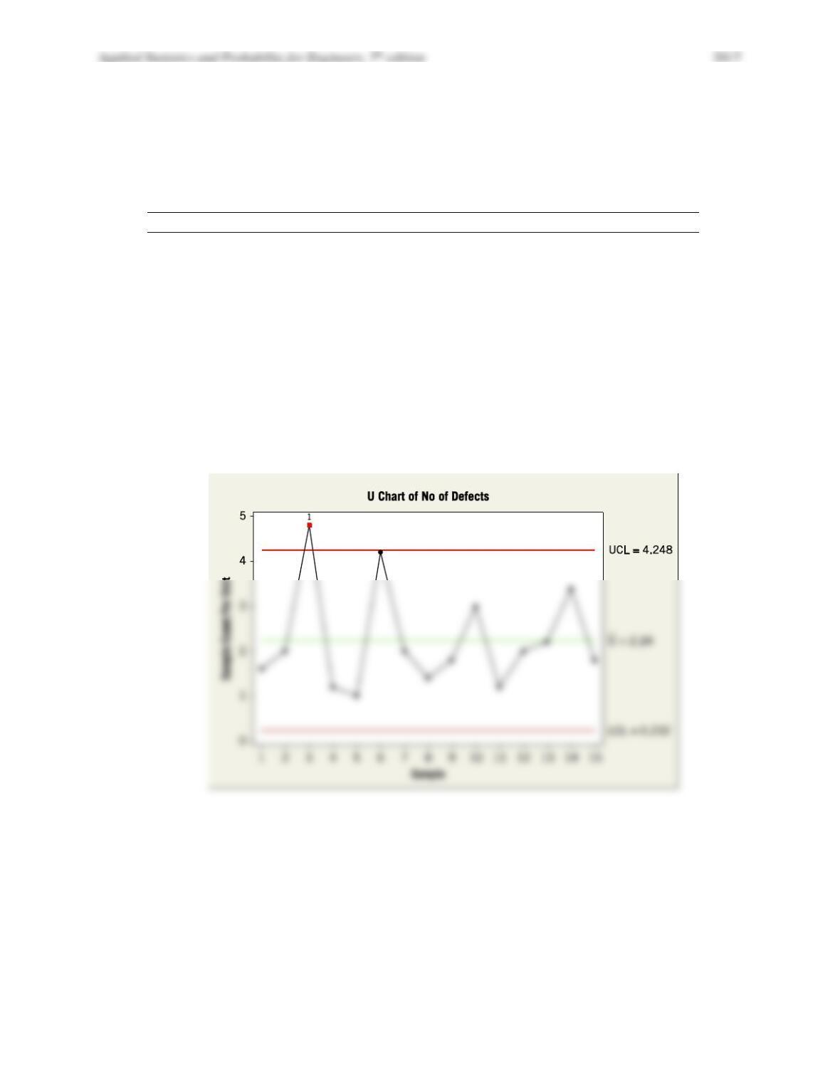
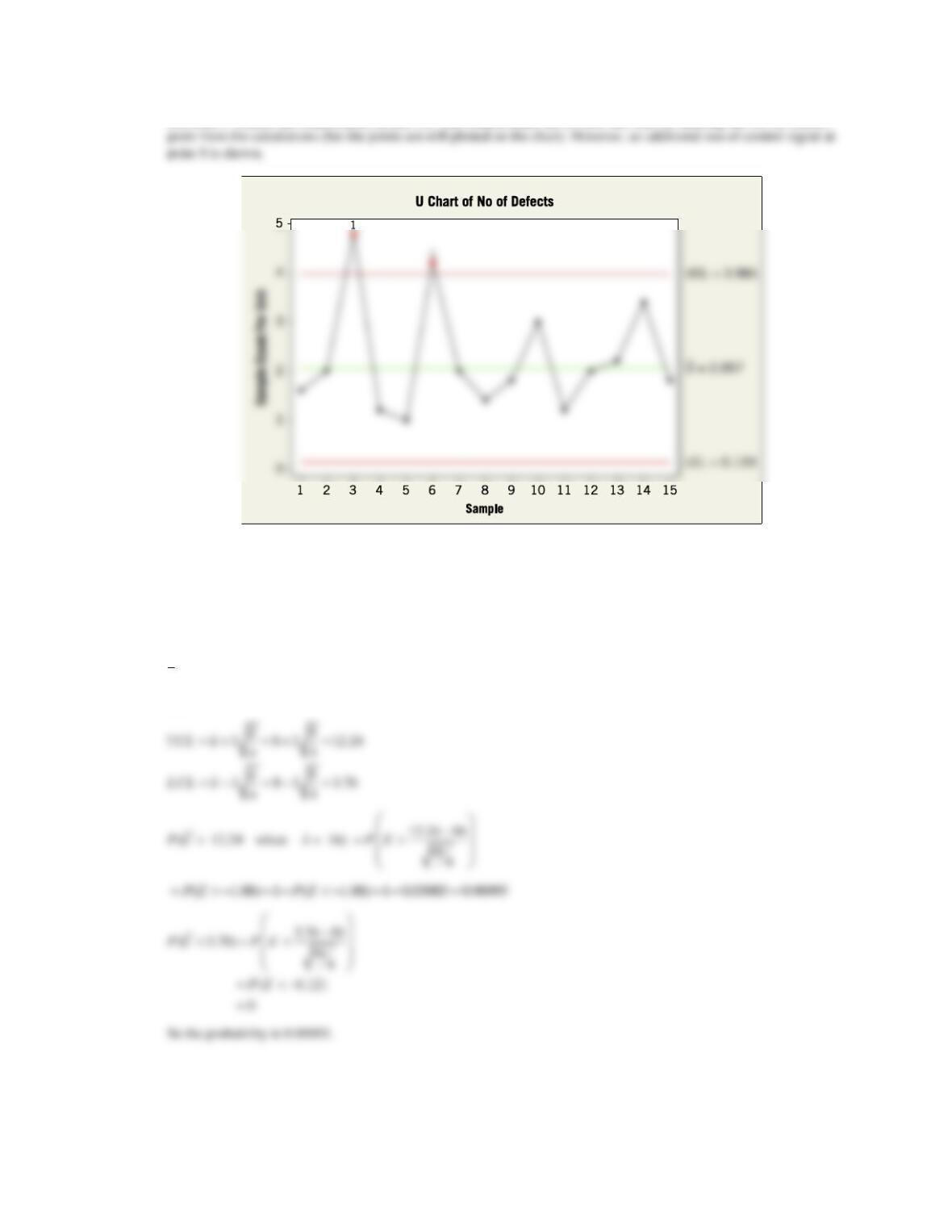
15.S24 The following are the number of defects observed on 15 samples of transmission units in an automotive manufacturing
company. Each lot contains five transmission units.
(a) Using all the data, compute trial control limits for a U control chart, construct the chart, and plot the data.
(b) Determine whether the process is in statistical control. If not, assume assignable causes can be found and out-of-
control points eliminated. Revise the control limits.
Sample
No. of Defects
Sample
No. of Defects
1
8
11
6
2
10
12
10
3
24
13
11
4
6
14
17
5
5
15
9
6
21
7
10
8
7
9
9
10
15
(a) The U chart follows.
Applied Statistics and Probability for Engineers, 7th edition 2017
15–69
(b) Point 3 violates the control limits in part (b). The control limits are revised one time by omitting the out-of-control
15.S25 Suppose that the average number of defects in a unit is known to be 8. If the mean number of defects in a unit shifts to
16, what is the probability that it is detected by a U chart on the first sample following the shift
(a) if the sample size is n = 4?
(b) if the sample size is n = 10?
Use a normal approximation for U.
8u=
(a) n = 4
Applied Statistics and Probability for Engineers, 7th edition 2017
15–70
(b) n = 10
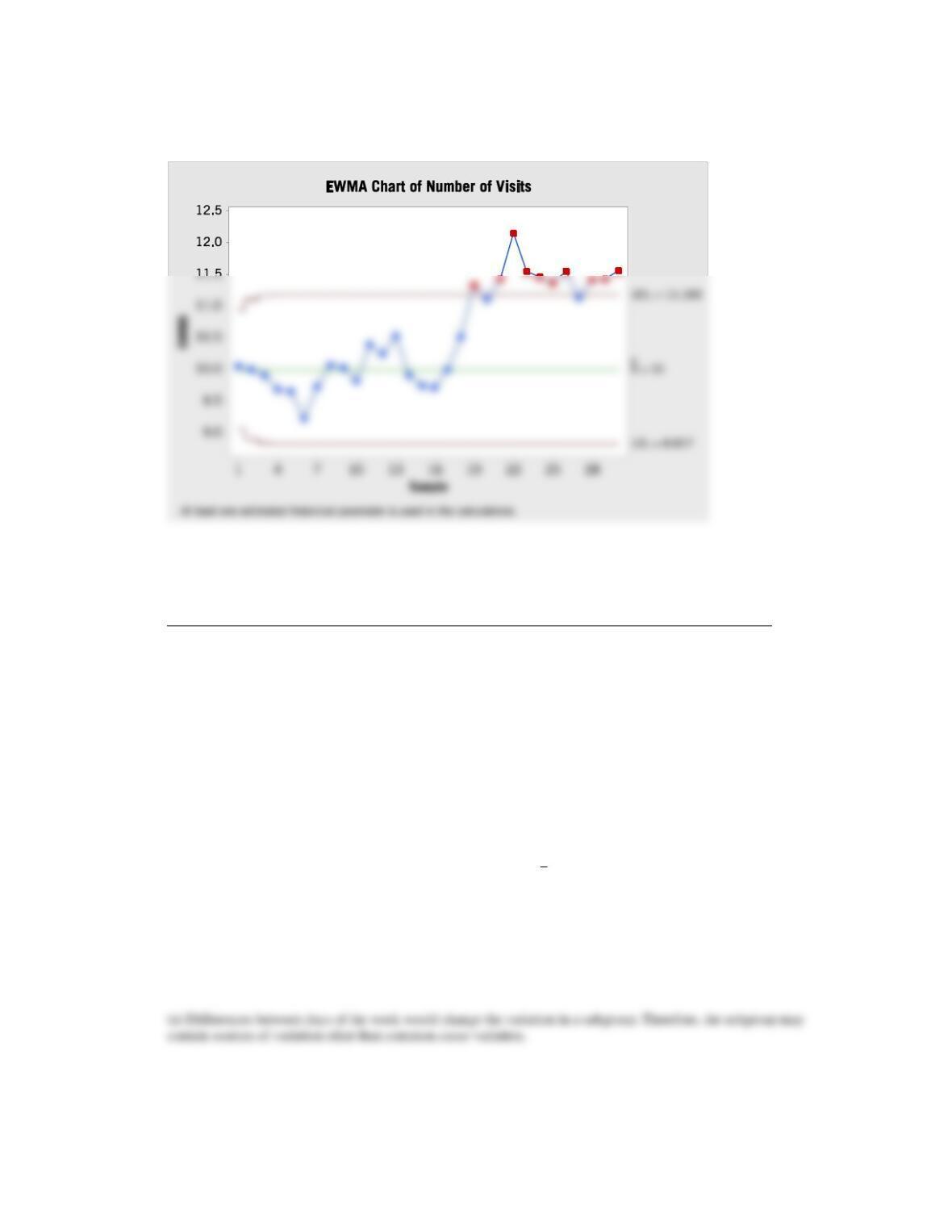
15.S26 The number of visits (in millions) on a Web site is recorded every day. The following table shows the samples for 25
consecutive days.
(a) Estimate the process standard estimation.
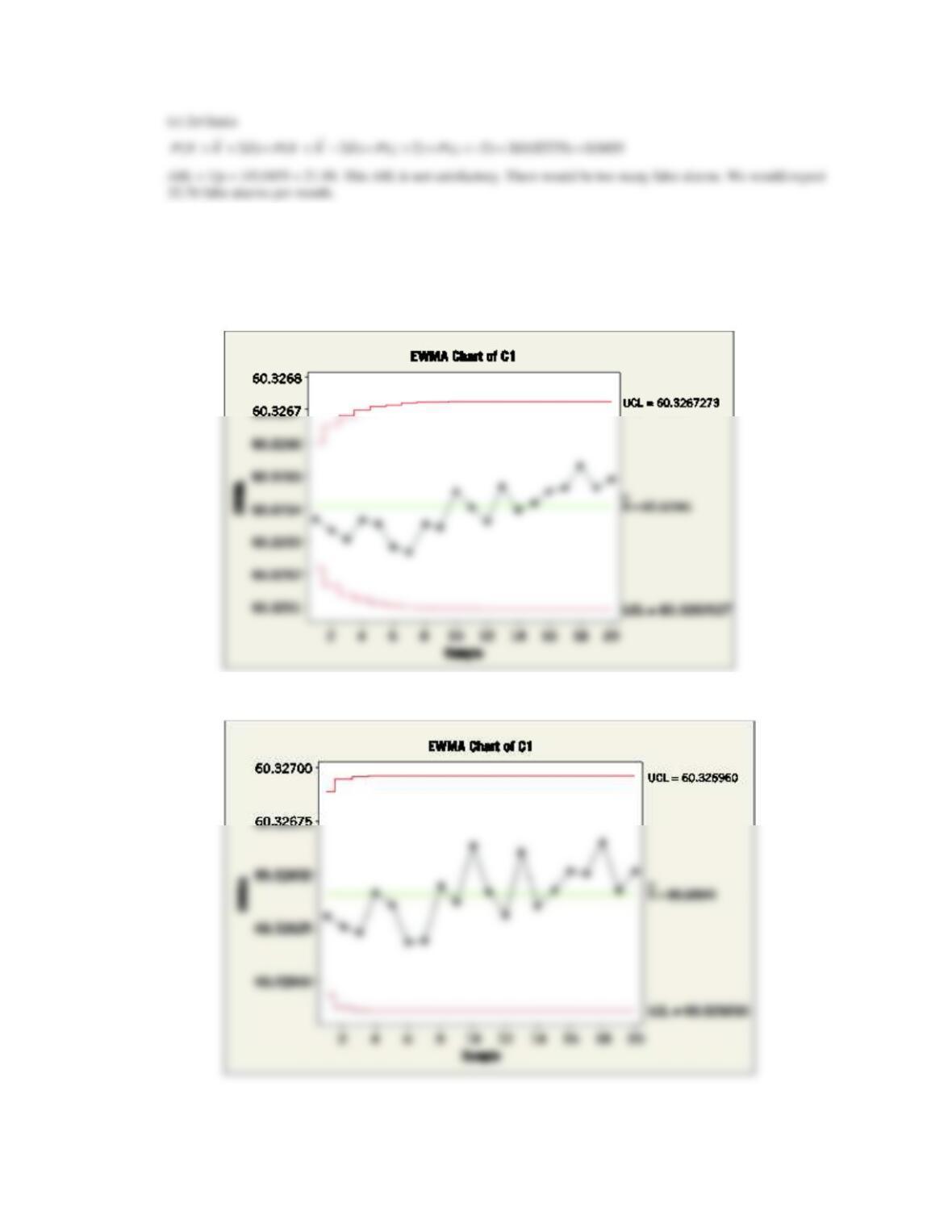
(b) Set up a EMWA control chart for this process, assuming the target is 10 with
= 0.4. Does the process appear to be
in control?
Sample
Number of Visits
Sample
Number of Visits
1
10.12
16
9.66
2
9.92
17
10.42
3
9.76
18
11.30
4
9.35
19
12.53
5
9.60
20
10.76
6
8.60
21
11.92
7
10.46
22
13.24
8
10.58
23
10.64
9
9.95
24
11.31
10
9.50
25
11.26
11
11.26
26
11.79
12
10.02
27
10.53
13
10.95
28
11.82
14
8.99
29
11.47
15
9.50
30
11.76
(a) Process standard deviation is estimated using the average moving range of size 2
Applied Statistics and Probability for Engineers, 7th edition 2017
15–71
(b) A EWMA chart with
= 0.4 and L = 3 follows. The process is not in control.
Set μ = 10 as the process mean.
15.S27 The following table shows the number of e-mails a student received each hour from 8:00 A.M. to 6:00 P.M.
The samples are collected for five days from Monday to Friday.
Hour
M
T
W
Th
F
1
2
2
2
3
1
2
2
4
0
1
2
3
2
2
2
1
2
4
4
4
3
3
2
5
1
1
2
2
1
6
1
3
2
2
1
7
3
2
1
1
0
8
2
3
2
3
1
9
1
3
3
2
0
10
2
3
2
3
0
(a) Use the rational subgrouping principle to comment on why an
X
chart that plots one point each hour with a
subgroup of size 5 is not appropriate.
(b) Construct an appropriate attribute control chart. Use all the data to find trial control limits, construct the chart, and
plot the data.
(c) Use the trial control limits from part (b) to identify out-of-control points. If necessary, revise your control limits,
assuming that any samples that plot outside the control limits can be eliminated.

Applied Statistics and Probability for Engineers, 7th edition 2017
15–72
(b) The data are ordered sequentially so that all hours in Monday are followed by all hours in Tuesday and so forth. In
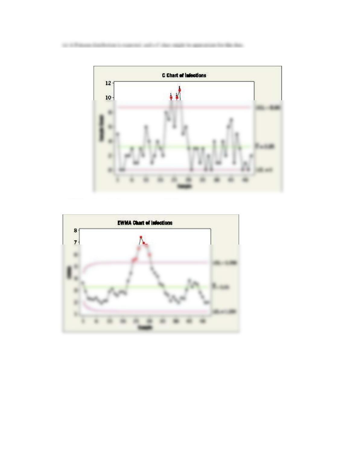
15.S28 A article in the Journal of Quality in Clinical Practice [“The Application of Statistical Process Control Charts to the
Detection and Monitoring of Hospital-Acquired Infections,” (2001, Vol. 21, pp. 112–117)] reported the use of SPC
methods to monitor hospital-acquired infections. The authors applied Shewhart and EWMA charts to the monitor
ESBL Klebsiella pneumonia infections. The monthly number of infections from June 1994 to April 1998 are shown in
the following table.
(a) What distribution might be expected for these data? What type of control chart might be appropriate?
(b) Construct the chart you selected in part (a).
Jan
Feb
Mar
April
May
Jun
Jul
Aug
Sep
Oct
Nov
Dec
1994
5
0
0
2
2
3
1
1995
1
3
2
6
4
1
2
4
3
2
8
7
1996
10
6
10
11
5
6
3
0
3
3
1
3
1997
0
2
0
4
1
1
4
2
6
7
1
5
1998
3
0
1
0
2
(c) Construct a EWMA chart for these data with
= 0.2. The article included a similarly constructed chart. What is
assumed for the distribution of the data in this chart? Can your EWMA chart perform adequately?
Applied Statistics and Probability for Engineers, 7th edition 2017
15–73
(b) For a C chart, signals occur at points 20, 21, and 22.
(c) EWMA with
= 0.2. Signals occur at points 20–26.

Applied Statistics and Probability for Engineers, 7th edition 2017
15–74
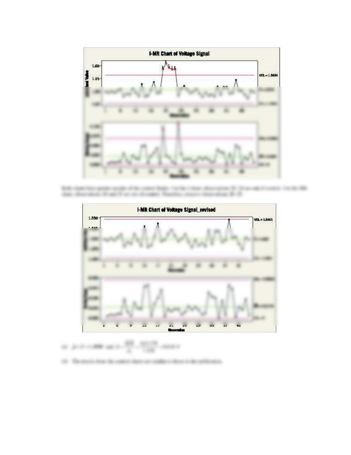
15.S29 An article in Microelectronics Reliability [“Advanced Electronic Prognostics through System Telemetry and Pattern
Recognition Methods,” (2007, 47(12), pp. 1865–1873)] presented an example of electronic prognostics (a technique
to detect faults in order to decrease the system downtime and the number of unplanned repairs in high-reliability and
high-availability systems). Voltage signals from enterprise servers were monitored over time. The measurements are
provided in the following table.
Observation
Voltage Signal
Observation
Voltage Signal
1
1.498
26
1.510
2
1.494
27
1.521
3
1.500
28
1.507
4
1.495
29
1.493
5
1.502
30
1.499
6
1.509
31
1.509
7
1.480
32
1.491
8
1.490
33
1.478
9
1.486
34
1.495
10
1.510
35
1.482
11
1.495
36
1.488
12
1.481
37
1.480
13
1.529
38
1.519
14
1.479
39
1.486
15
1.483
40
1.517
16
1.505
41
1.517
17
1.536
42
1.490
18
1.493
43
1.495
19
1.496
44
1.545
20
1.587
45
1.501
21
1.610
46
1.503
22
1.592
47
1.486
23
1.585
48
1.473
24
1.587
49
1.502
25
1.482
50
1.497
(a) Using all the data, compute trial control limits for individual observations and moving-range charts. Construct the
chart and plot the data. Determine whether the process is in statistical control. If not, assume that assignable
causes can be found to eliminate these samples and revise the control limits.
(b) Estimate the process mean and standard deviation for the in-control process.
(c) The report in the article assumed that the signal is normally distributed with a mean of 1.5 V and a standard
deviation of 0.02 V. Do your results in part (b) support this assumption?
Applied Statistics and Probability for Engineers, 7th edition 2017
15–75
(a)
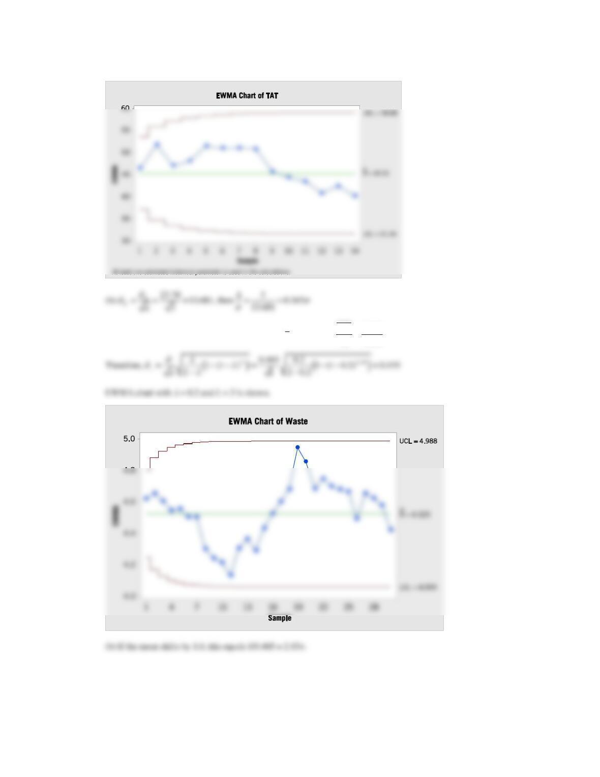
15.S30 Consider the turnaround time (TAT) for complete blood counts in Exercise 15.3.12. Suppose that the specifications for
TAT are set at 20 and 80 minutes. Use the control chart summary statistics for the following.
(a) Estimate the process standard deviation.
(b) Calculate PCR and PCRk for the process.’
Applied Statistics and Probability for Engineers, 7th edition 2017
15–76
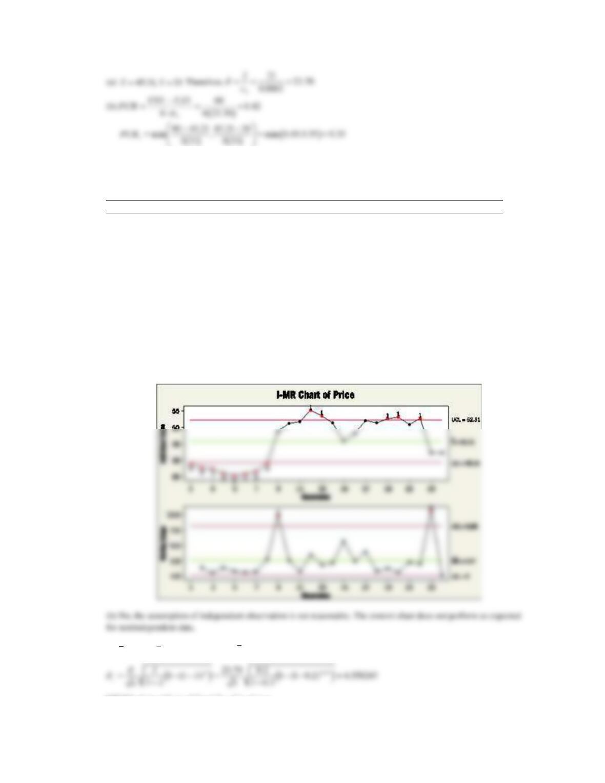
15.S31 An article in Electric Power Systems Research [“On the Self-Scheduling of a Power Producer in Uncertain Trading
Environments” (2008, 78(3), pp. 311–317)] considered a self-scheduling approach for a power producer. The following
table shows the forecasted prices of energy for a 24-hour time period according to a base case scenario.
Hour
Price
Hour
Price
Hour
Price
1
38.77
9
48.75
17
52.07
2
37.52
10
51.18
18
51.34
3
37.07
11
51.79
19
52.55
4
35.82
12
55.22
20
53.11
5
35.04
13
53.48
21
50.88
6
35.57
14
51.34
22
52.78
7
36.23
15
45.8
23
42.16
8
38.93
16
48.14
24
42.16
(a) Construct individuals and moving-range charts. Determine whether the energy prices fluctuate in statistical control.
(b) Is the assumption of independent observations reasonable for these data?
(a) The control charts indicate the process is not in control.
15.S32 (a)
45.21,x=
21s=
. Therefore,
4
ˆ/ 21/ 0.8862 23.70sc
= = =
EWMA chart with
= 0.2 and L = 3 is shown.
Applied Statistics and Probability for Engineers, 7th edition 2017
15–77
15.S33 (a) From the individuals and moving range charts,
4.523x=
2
0.524
ˆ0.465
1.128
MR
d
= =