
14-61
14.11.5 An article in Tappi (1960, Vol. 43, pp. 38–44) describes an experiment that investigated the ash value of paper pulp (a
measure of inorganic impurities). Two variables, temperature T in degrees Celsius and time t in hours, were studied,
and some of the results are shown in the following table. The coded predictor variables shown are
−−
==
12
( 775) ( 3)
,
115 1.5
Tt
xx
and the response y is (dry ash value in %) × 103.
x1
x2
y
x1
x2
y
−1
−1
211
0
−1.5
168
1
−1
92
0
1.5
179
−1
1
216
0
0
122
1
1
99
0
0
175
−1.5
0
222
0
0
157
1.5
0
48
0
0
146
(a) What type of design has been used in this study? Is the design rotatable?
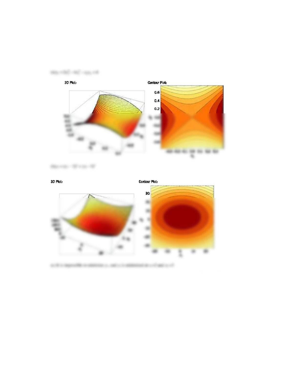
(b) Fit a quadratic model to the data. Is this model satisfactory?
(c) If it is important to minimize the ash value, where would you run the process?
(b) Term Coef StDev T P
Constant 150.04 7.821 19.184 0.000
x1 -58.47 5.384 -10.861 0.000
Analysis of Variance for y
Source DF Seq SS Adj SS Adj MS F P
Regression 5 30688.7 30688.7 6137.7 24.91 0.001
Linear 2 29155.4 29155.4 14577.7 59.17 0.000
14.11.6 In their book Empirical Model Building and Response Surfaces (John Wiley, 1987), Box and Draper described an
experiment with three factors. The data in the following table are a variation of the original experiment from their book.
Suppose that these data were collected in a semiconductor manufacturing process.
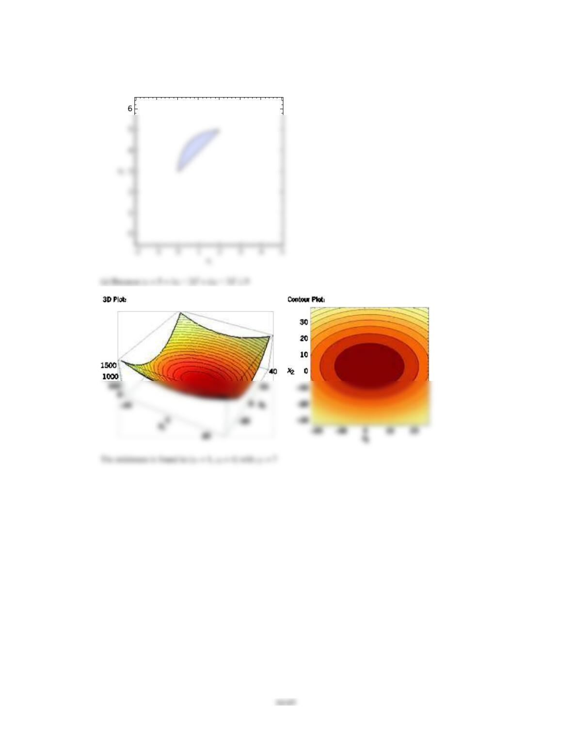
(a) The response y1 is the average of three readings on resistivity for a single wafer. Fit a quadratic model to this
response.

Applied Statistics and Probability for Engineers, 7th edition 2017
14-62
(b) The response y2 is the standard deviation of the three resistivity measurements. Fit a linear model to this response.
(c) Where would you recommend that we set x1, x2, and x3 if the objective is to hold mean resistivity at 500 and
minimize the standard deviation?
x1
x2
x3
y1
y2
−1
−1
−1
24.00
12.49
0
−1
−1
120.33
8.39
1
−1
−1
213.67
42.83
−1
0
−1
86.00
3.46
0
0
−1
136.63
80.41
1
0
−1
340.67
16.17
−1
1
−1
112.33
27.57
0
1
−1
256.33
4.62
1
1
−1
271.67
23.63
−1
−1
0
81.00
0.00
0
−1
0
101.67
17.67
1
−1
0
357.00
32.91
−1
0
0
171.33
15.01
0
0
0
372.00
0.00
1
0
0
501.67
92.50
−1
1
0
264.00
63.50
0
1
0
427.00
88.61
1
1
0
730.67
21.08
−1
−1
1
220.67
133.82
0
−1
1
239.67
23.46
1
−1
1
422.00
18.52
−1
0
1
199.00
29.44
0
0
1
485.33
44.67
1
0
1
673.67
158.21
−1
1
1
176.67
55.51
0
1
1
501.00
138.94
1
1
1
1010.00
142.45
(a) Response Surface Regression
Estimated Regression Coefficients for y
Term Coef SE Coef T P
Constant 327.62 38.76 8.453 0.000
x3 131.47 17.94 7.328 0.000
x2 109.43 17.94 6.099 0.000
x1 177.00 17.94 9.866 0.000
Analysis of Variance for y
Source DF Seq SS Adj SS Adj MS F P
Regression 9 1248237 1248237 138693 23.94 0.000
Linear 3 1090558 1090558 363519 62.74 0.000

Applied Statistics and Probability for Engineers, 7th edition 2017
14-63
Reduced model:
Term Coef SE Coef T P
Constant 314.67 15.46 20.354 0.000
1 1 2 3 1 2 1 3
(b) Response Surface Regression
Estimated Regression Coefficients for y2
Term Coef SE Coef T P
Constant 48.00 7.808 6.147 0.000
Analysis of Variance for y2
Source DF Seq SS Adj SS Adj MS F P
Regression 3 21957.3 21957.3 7319.09 4.45 0.013
(c) The equations for y1 and y2 are used to determine values for the x’s. Given values for x1 and x2, a value for x3 can be
solved to set y1 to a target. Each xi should range from −1 to 1 to stay within the experimental region for the models. The
14.11.7 Consider the first-order model
= + − + −
1 2 3 4
12 1.2 2.1 1.6 0.6y x x x x
where −1 ≤ xi ≤ 1.
(a) Find the direction of steepest ascent.
(b) Assume that the current design is centered at the point (0,0,0,0). Determine the point that is three units from the
current center point in the direction of steepest ascent.
Applied Statistics and Probability for Engineers, 7th edition 2017
14-64
14.11.8 Suppose that a response y1 is a function of two inputs x1 and x2 with
= − − +
22
1 2 1 1 2
2 4 4y x x x x
.
(a) Draw the contours of this response function.
(b) Consider another response y2 = (x1 − 2)2 + (x2 − 3)2.
(c) Add the contours for y2 and discuss how feasible it is to minimize both y1 and y2 with values for x1 and x2.
14.11.9 Two responses y1 and y2 are related to two inputsx1 and x2 by the models y1 = 5 + (x1 − 2)2+(x2 − 3)2 and y2 = x2 −
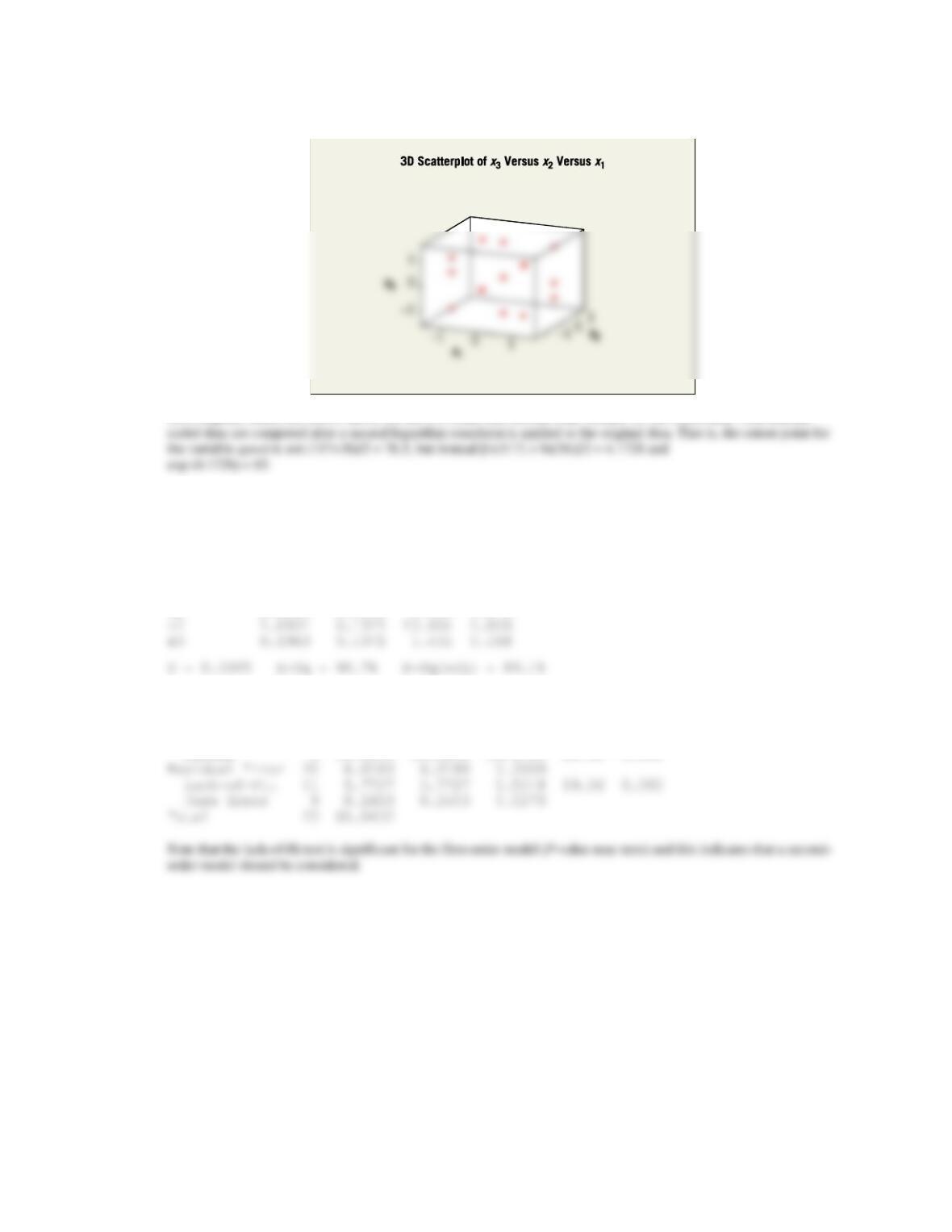
x1 + 3.Suppose that the objectives are y1 ≤ 9 and y2≥ 6.
(a) Is there a feasible set of operating conditions for x1 and x2? If so, plot the feasible region in the space of x1 and x2.
(b) Determine the point(s) (x1, x2) that yields y2 ≥ 6 and minimizes y1.
= − − +
22
2 4 4y x x x x
Applied Statistics and Probability for Engineers, 7th edition 2017
(a) The region y1 < 9 is a circle in (x1, x2) space centered as the point (2,3) with radius 2. The region y2> 6 is the half
plane x2 >x1 + 3. The following graph shows the feasible region.

14-66
14.11.10 An article in the Journal of Materials Processing Technology (1997, Vol. 67, pp. 55–61) used response surface
methodology to generate surface roughness prediction models for turning EN 24T steel (290 BHN). The data are shown
in the following table.
Trial
Speed
(m min−1)
Feed
(mm rev−1)
Depth
of cut
(mm)
Coding
Surface
roughness,
(μm)
x1
x2
x3
1
36
0.15
0.50
−1
−1
−1
1.8
2
117
0.15
0.50
1
−1
−1
1.233
3
36
0.40
0.50
−1
1
−1
5.3
4
117
0.40
0.50
1
1
−1
5.067
5
36
0.15
1.125
−1
−1
1
2.133
6
117
0.15
1.125
1
−1
1
1.45
7
36
0.40
1.125
−1
1
1
6.233
8
117
0.40
1.125
1
1
1
5.167
9
65
0.25
0.75
0
0
0
2.433
10
65
0.25
0.75
0
0
0
2.3
11
65
0.25
0.75
0
0
0
2.367
12
65
0.25
0.75
0
0
0
2.467
13
28
0.25
0.75
−2
0
0
3.633
14
150
0.25
0.75
2
0
0
2.767
15
65
0.12
0.75
0
−2
0
1.153
16
65
0.50
0.75
0
2
0
6.333
17
65
0.25
0.42
0
0
−2
2.533
18
65
0.25
1.33
0
0
2
3.20
19
28
0.25
0.75
−2
0
0
3.233
20
150
0.25
0.75
2
0
0
2.967
21
65
0.12
0.75
0
−2
0
1.21
22
65
0.50
0.75
0
2
0
6.733
23
65
0.25
0.42
0
0
−2
2.833
24
65
0.25
1.33
0
0
2
3.267
The factors and levels for the experiment are shown in Table E14-3.
TABLE E14-3 Steel Factors
Levels
Lowest
Low
Center
High
Highest
Coding
−2
−1
0
1
2
Speed, V (m min−1)
28
36
65
117
150
Feed, f (mm rev−1)
0.12
0.15
0.25
0.40
0.50
Depth of cut, d (mm)
0.42
0.50
0.75
1.125
1.33
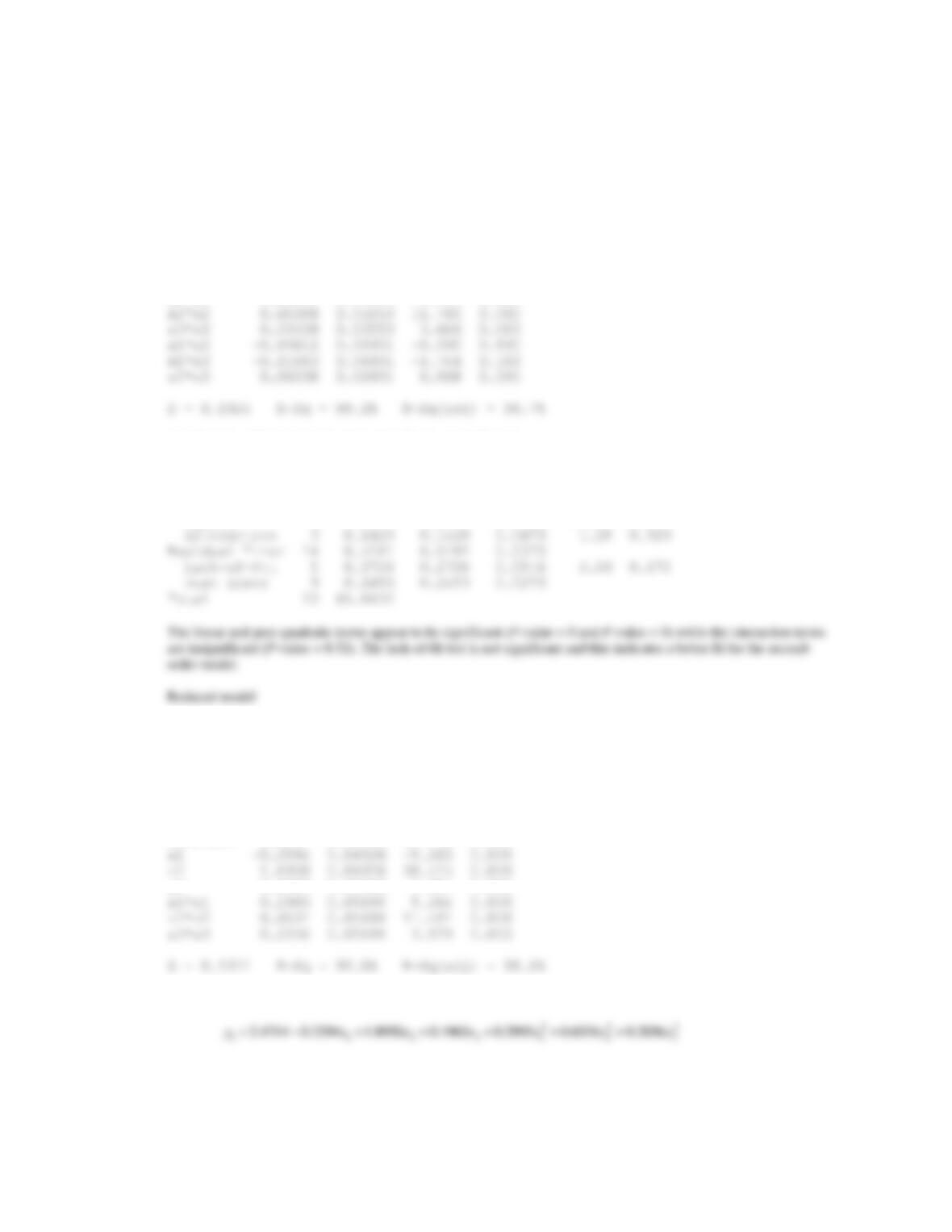
(a) Plot the points at which the experimental runs were made.
(b) Fit both first-and second-order models to the data. Comment on the adequacies of these models.
(c) Plot the roughness response surface for the second-order model and comment.
Applied Statistics and Probability for Engineers, 7th edition 2017
14-67
(a) A plot of the coded data follows.
(b) Computer results are shown below for the first-order and second-order models for the coded data. Note that the
Response Surface Regression: y Versus x1, x2, x3
The analysis was done using coded units.
Estimated Regression Coefficients for y
Term Coef SE Coef T P
Constant 3.2422 0.1120 28.955 0.000
x1 -0.2594 0.1371 -1.891 0.073
Analysis of Variance for y
Source DF Seq SS Adj SS Adj MS F P
Regression 3 59.0253 59.0253 19.6751 65.39 0.000
Linear 3 59.0253 59.0253 19.6751 65.39 0.000
Applied Statistics and Probability for Engineers, 7th edition 2017
14-68
Response Surface Regression: Surface Roughness Versus x1, x2, x3
The analysis was done using coded units.
Estimated Regression Coefficients for Surface Roughness
Term Coef SE Coef T P
Constant 2.47142 0.08780 28.147 0.000
x1 -0.25937 0.04809 -5.393 0.000
x2 1.89296 0.04809 39.361 0.000
x3 0.19625 0.04809 4.081 0.001
x1*x1 0.29946 0.05553 5.393 0.000
Analysis of Variance for Surface Roughness
Source DF Seq SS Adj SS Adj MS F P
Regression 9 64.5252 64.5252 7.1695 193.74 0.000
Linear 3 59.0252 59.0252 19.6751 531.67 0.000
Square 3 5.3579 5.3579 1.7860 48.26 0.000
Response Surface Regression: Roughness Versus x1, x2, x3
The analysis was done using coded units.
Estimated Regression Coefficients for Roughness
Term Coef SE Coef T P
Constant 2.4714 0.08994 27.478 0.000
x3 0.1963 0.04926 3.984 0.001
The quadratic model of the coded variable is
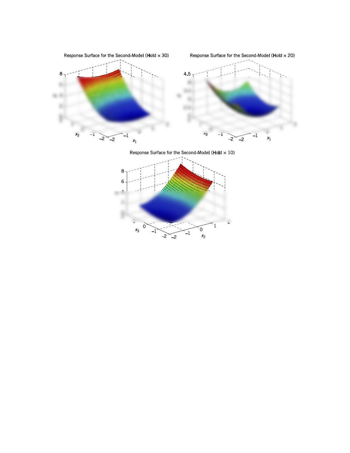
Applied Statistics and Probability for Engineers, 7th edition 2017
14-69
(c) There is curvature in the fitted surface from the second-order effects.

Applied Statistics and Probability for Engineers, 7th edition 2017
14-70
14.11.11 An article in Analytical Biochemistry [“Application of Central Composite Design for DNA Hybridization
Onto Magnetic Microparticles,” (2009, Vol. 391(1), 2009, pp. 17–23)] considered the effects of probe and target
concentration and particle number in immobilization and hybridization on a micro particle-based DNA hybridization
assay. Mean fluorescence is the response. Particle concentration was transformed to surface area measurements. Other
concentrations were measured in micromoles per liter (μM). Data are in Table E14-2.
TABLE E14-2 Fluorescence Experiment
Run
Immobilization
Area (cm2)
Probe
Area (μM)
Hybridization
(cm2)
Target (μM)
Mean
Fluorescence
1
0.35
0.025
0.35
0.025
4.7
2
7
0.025
0.35
0.025
4.7
3
0.35
2.5
0.35
0.025
28.0
4
7
2.5
0.35
0.025
81.2
5
0.35
0.025
3.5
0.025
5.7
6
7
0.025
3.5
0.025
3.8
7
0.35
2.5
3.5
0.025
12.2
8
7
2.5
3.5
0.025
19.5
9
0.35
0.025
0.35
5
4.4
10
7
0.025
0.35
5
2.6
11
0.35
2.5
0.35
5
83.7
12
7
2.5
0.35
5
84.7
13
0.35
0.025
3.5
5
6.8
14
7
0.025
3.5
5
2.4
15
0.35
2.5
3.5
5
76
16
7
2.5
3.5
5
77.9
17
0.35
5
2
2.5
42.6
18
7
5
2
2.5
52.3
19
3.5
0.025
2
2.5
2.6
20
3.5
2.5
2
2.5
72.8
21
3.5
5
0.35
2.5
47.7
22
3.5
5
3.5
2.5
54.4
23
3.5
5
2
0.025
30.8
24
3.5
5
2
5
64.8
25
3.5
5
2
2.5
51.6
26
3.5
5
2
2.5
52.6
27
3.5
5
2
2.5
56.1
(a) What type of design is used?
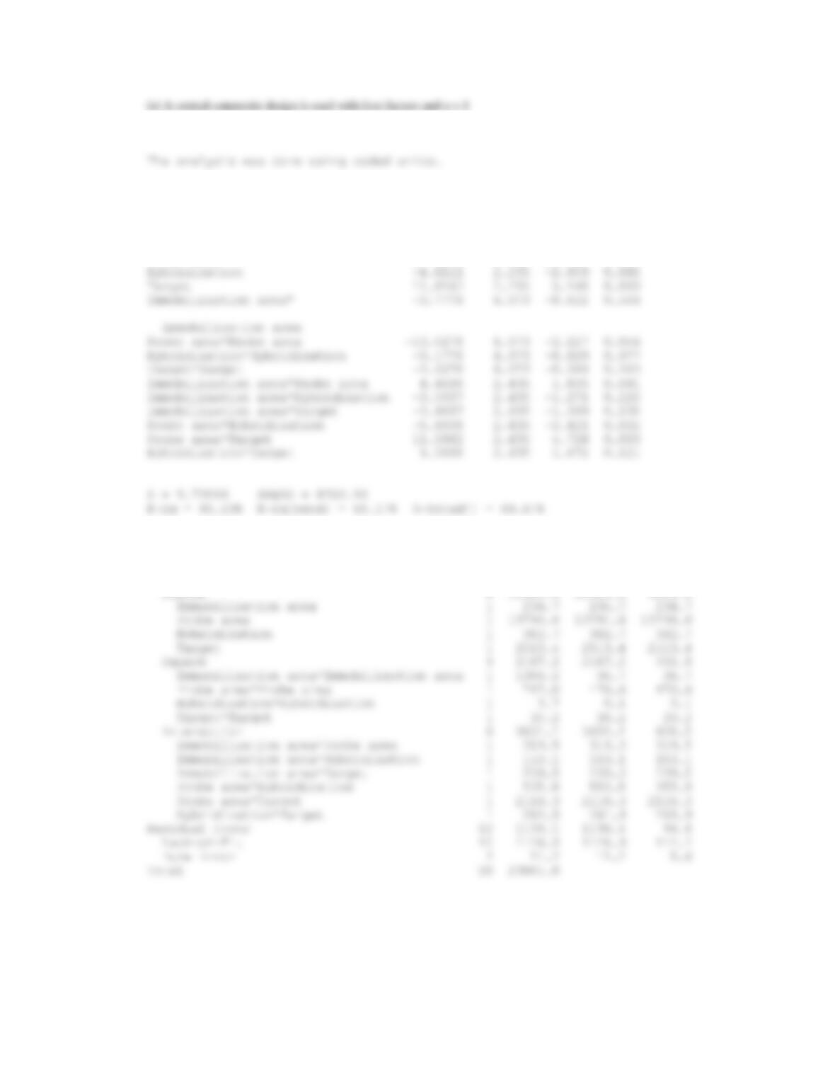
(b) Fit a second-order response surface model to the data.
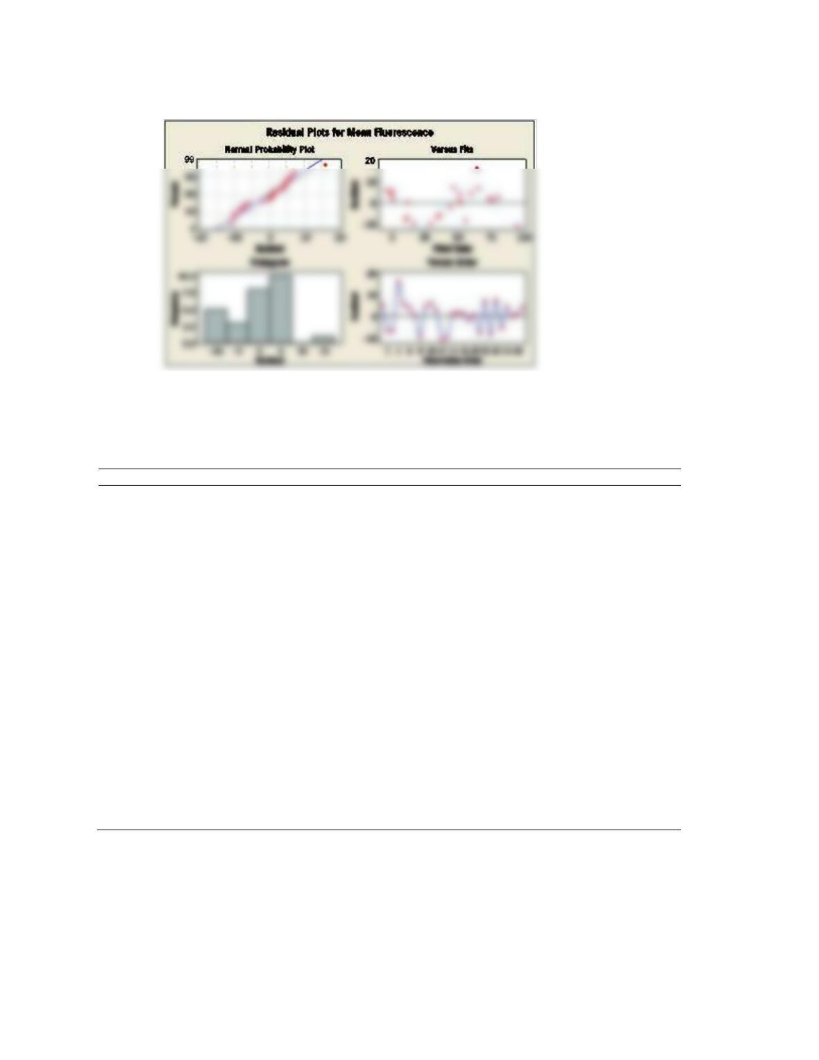
(c) Does a residual analysis indicate any problems?
Applied Statistics and Probability for Engineers, 7th edition 2017
14-71
(b)
Estimated Regression Coefficients for Mean fluorescence
Term Coef SE Coef T P
Constant 51.9630 3.589 14.479 0.000
Immobilization area 3.6111 2.295 1.573 0.142
Probe area 27.6833 2.295 12.060 0.000
Analysis of Variance for Mean fluorescence
Source DF Seq SS Adj SS Adj MS
Regression 14 22743.7 22743.7 1624.6
Linear 4 16925.5 16925.5 4231.4
Applied Statistics and Probability for Engineers, 7th edition 2017
14-72
(c) The residual plots do not indicate any problems.
14.11.12 An article in Applied Biochemistry and Biotechnology (“A Statistical Approach for Optimization of
Polyhydroxybutyrate Production by Bacillus sphaericus NCIM 5149 under Submerged Fermentation Using Central
Composite Design” (2010, Vol. 162(4), pp. 996–1007)] described an experiment to optimize the production of
polyhydroxybutyrate (PHB). Inoculum age, pH, and substrate were selected as factors, and a central composite design
was conducted. Data follow.
Run
Inoculum age (h)
pH
Substrate (g/L)
PHB (g/L)
1
12
4
1
0.84
2
24
8
1
0.55
3
18
6
2.5
1.96
4
28
6
2.5
1.2
5
12
4
4
0.783
6
18
6
2.5
1.66
7
18
6
2.5
2.22
8
18
6
5
0.8
9
12
8
4
0.48
10
18
6
2.5
1.97
11
18
6
2.5
2.2
12
18
6
2.5
2.25
13
18
2
2.5
0.2
14
18
6
0
0.22
15
12
8
1
0.37
16
24
8
4
0.66
17
24
4
1
0.28
18
24
4
4
0.88
19
18
9
2.5
0.3
20
7
6
2.5
0.42
(a) Plot the points at which the experimental runs were made [Hint: Code each variable first.] What type of design is
used?
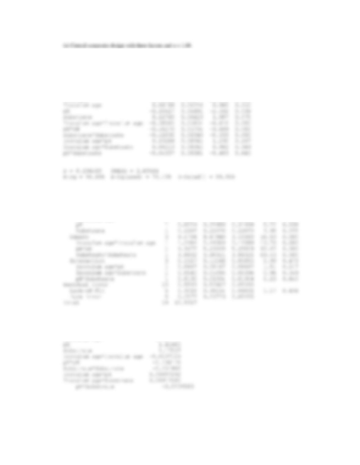
(b) Fit a second-order response surface model to the data.
(c) Does a residual analysis indicate any problems?
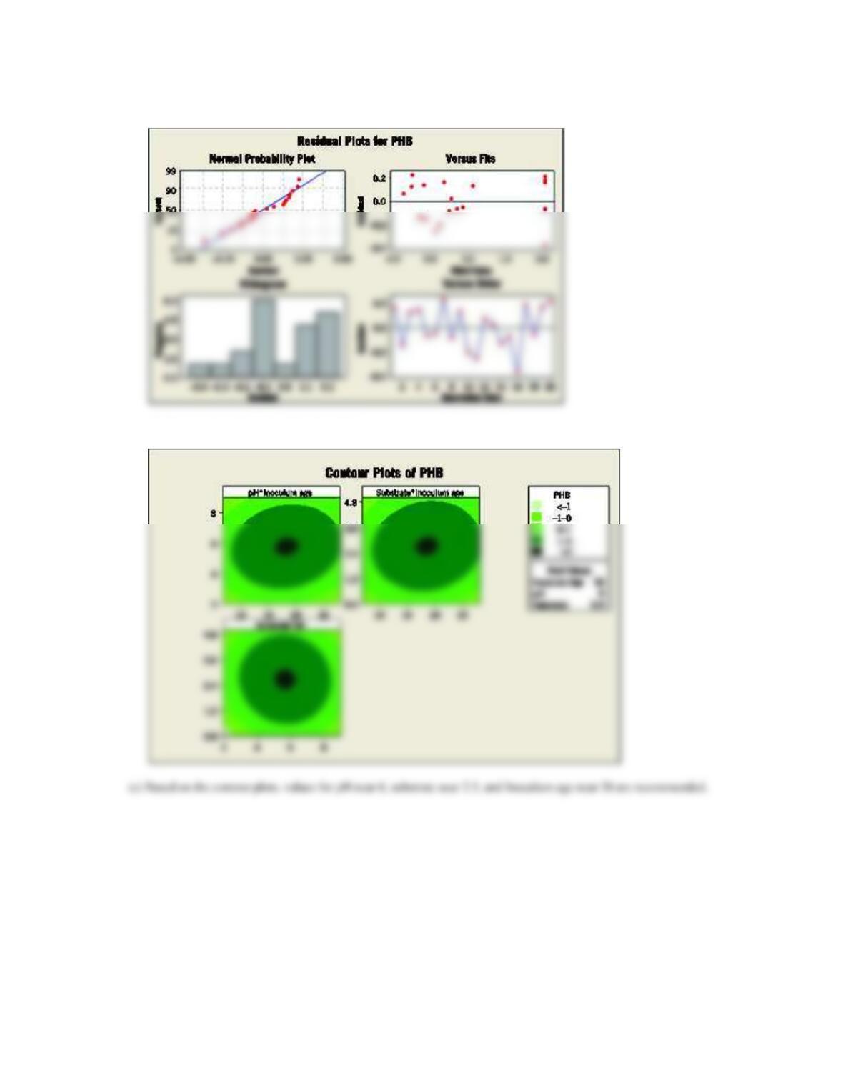
(d) Construct a contour plot and response surface for PHB amount in terms of two factors.
(e) Can you recommend values for inoculum age, pH, and substrate to maximize production?
Applied Statistics and Probability for Engineers, 7th edition 2017
14-73
(b)
The analysis was done using coded units.
Estimated Regression Coefficients for PHB
Term Coef SE Coef T P
Constant 2.03328 0.09577 21.232 0.000
Analysis of Variance for PHB
Source DF Seq SS Adj SS Adj MS F P
Regression 9 9.9725 9.97247 1.10805 19.81 0.000
Linear 3 0.3414 0.59413 0.19804 3.54 0.056
Inoculum age 1 0.1187 0.05368 0.05368 0.96 0.350
Estimated Regression Coefficients for PHB using data in uncoded units
Term Coef
Constant -6.67722
Inoculum age 0.321711
Applied Statistics and Probability for Engineers, 7th edition 2017
14-74
(c) Residual plots for the reduced model.
(d) Contour plots from the reduced model.

Applied Statistics and Probability for Engineers, 7th edition 2017
14-75
Supplemental Exercises
14.S6 Heat-treating metal parts is a widely used manufacturing process. An article in the Journal of Metals (1989,
Vol. 41) described an experiment to investigate flatness distortion from heat-treating for three types of gears
and two heat-treating times. The data follow:
Gear Type
Time (minutes)
90
120
20-tooth
0.0265
0.0560
0.0340
0.0650
24-tooth
0.0430
0.0720
0.0510
0.0880
28-tooth
0.0405
0.0620
0.0575
0.0825
(a) Is there any evidence that flatness distortion is different for the different gear types? Is there any indication that
heat-treating time affects the flatness distortion? Do these factors interact? Use
= 0.05.
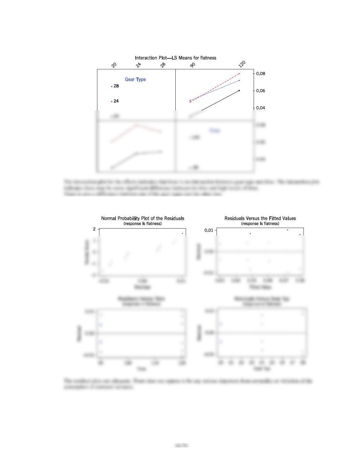
(b) Construct graphs of the factor effects that aid in drawing conclusions from this experiment.
(c) Analyze the residuals from this experiment. Comment on the validity of the underlying assumptions.
(a)
Factor Type Levels Values
Gear Typ fixed 3 20 24 28
Term Coef SE Coef T P
Constant 0.056500 0.002846 19.85 0.000
Gear Typ
20 -0.011125 0.004025 -2.76 0.033
Applied Statistics and Probability for Engineers, 7th edition 2017
(b)
(c) The model used is
= = −
12
ˆ0.0565 0.0111 0.01144y x x
14-77
14.S7 An article in Process Engineering (1992, No. 71, pp. 46–47) presented a two-factor factorial experiment to investigate
the effect of pH and catalyst concentration on product viscosity (cSt). The data are as follows:
pH
Catalyst Concentration
2.5
2.7
5.6
192, 199, 189, 198
178, 186, 179, 188
5.9
185, 193, 185, 192
197, 196, 204, 204
(a) Test for main effects and interactions using
= 0.05. What are your conclusions?
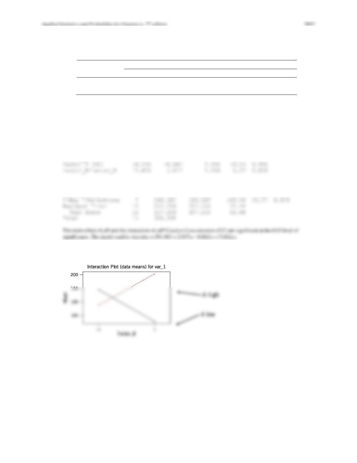
(b) Graph the interaction and discuss the information provided by this plot.
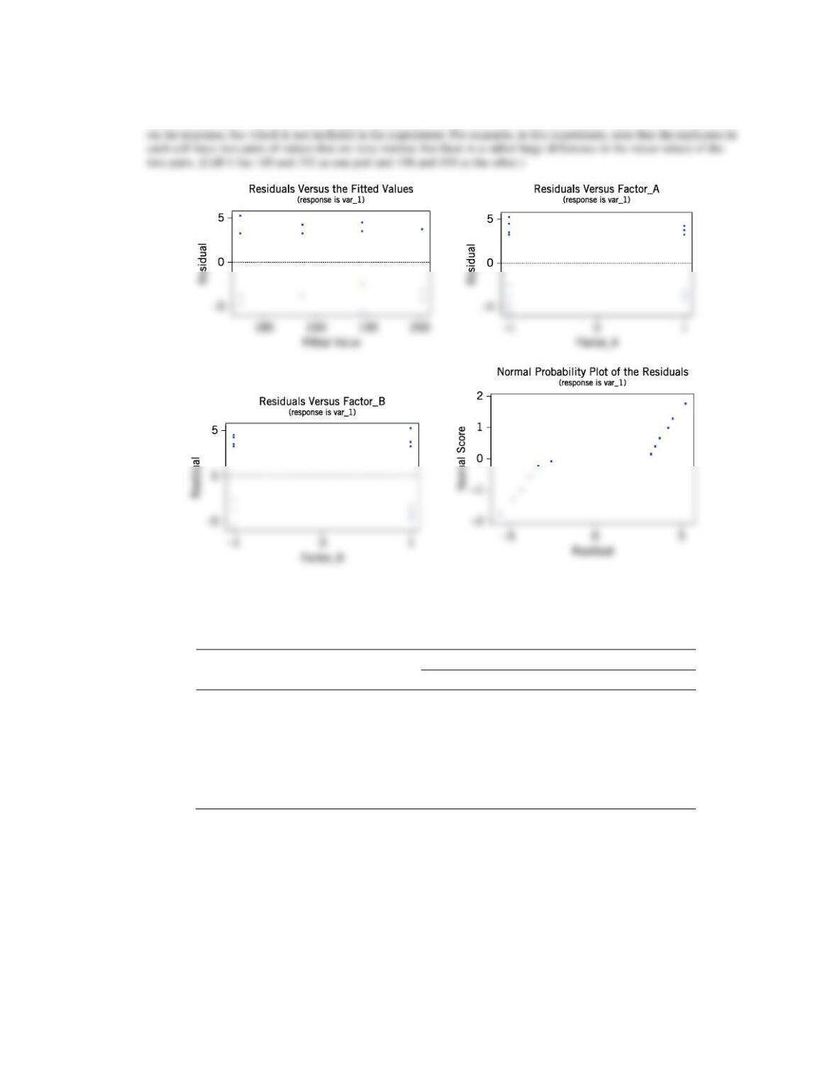
(c) Analyze the residuals from this experiment.
(a) Estimated Effects and Coefficients for var_1 (coded units)
Term Effect Coef SE Coef T P
Constant 191.563 1.158 165.49 0.000
factor_A (PH) 5.875 2.937 1.158 2.54 0.026
Analysis of Variance for var_1 (coded units)
Source DF Seq SS Adj SS Adj MS F P
Main Effects 2 138.125 138.125 69.06 3.22 0.076
(b) The interaction plot shows that there is a strong interaction. When Factor A is at its low level, the mean response is
large at the low level of B and is small at the high level of B. However, when A is at its high level, the results reverse.
Applied Statistics and Probability for Engineers, 7th edition 2017
14-78
(c) The plots of the residuals show that the equality of variance assumption is reasonable. However, there is a large gap
in the middle of the normal probability plot. Sometimes, this can indicate that there is another variable that has an effect
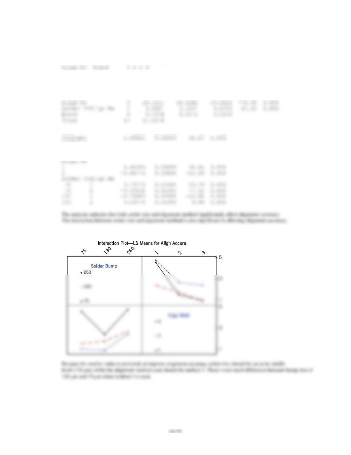
14.S8 An article in the IEEE Transactions on Components, Hybrids, and Manufacturing Technology (1992, Vol. 15)
described an experiment for aligning optical chips onto circuit boards. The method involves placing solder bumps onto
the bottom of the chip. The experiment used three solder bump sizes and three alignment methods. The response
variable is alignment accuracy (in micrometers). The data are as follows:
Solder Bump Size (diameter in mm)
Alignment Method
1
2
3
4.60
1.55
1.05
75
4.53
1.45
1.00
2.33
1.72
0.82
130
2.44
1.76
0.95
4.95
2.73
2.36
260
4.55
2.60
2.46
(a) Is there any indication that either solder bump size or alignment method affects the alignment accuracy? Is there any
evidence of interaction between these factors? Use
= 0.05.
(b) What recommendations would you make about this process?
(c) Analyze the residuals from this experiment. Comment on model adequacy.
Applied Statistics and Probability for Engineers, 7th edition 2017
(a)
Factor Type Levels Values
Solder B fixed 3 75 130 260
Analysis of Variance for Align Ac, using Adjusted SS for Tests
Source DF Seq SS Adj SS Adj MS F P
Solder B 2 7.7757 7.7757 3.8879 297.92 0.000
Term Coef SE Coef T P
Solder B
75 -0.07278 0.03808 -1.91 0.088
130 -0.76611 0.03808 -20.12 0.000
(b) The lines for factor A intersect at the lower level of alignment.