Applied Statistics and Probability for Engineers, 7th edition 2017
14-1
CHAPTER 14
Section 14.3
14.3.1 An article in Industrial Quality Control (1956, pp. 5 – 8) describes an experiment to investigate the effect of two
factors (glass type and phosphor type) on the brightness of a television tube. The response variable measured
is the current (in microamps) necessary to obtain a specified brightness level. The data are shown in the
following table:
(a) State the hypotheses of interest in this experiment.
(b) Test the hypotheses in part (a) and draw conclusions using the analysis of variance with
= 0.05.
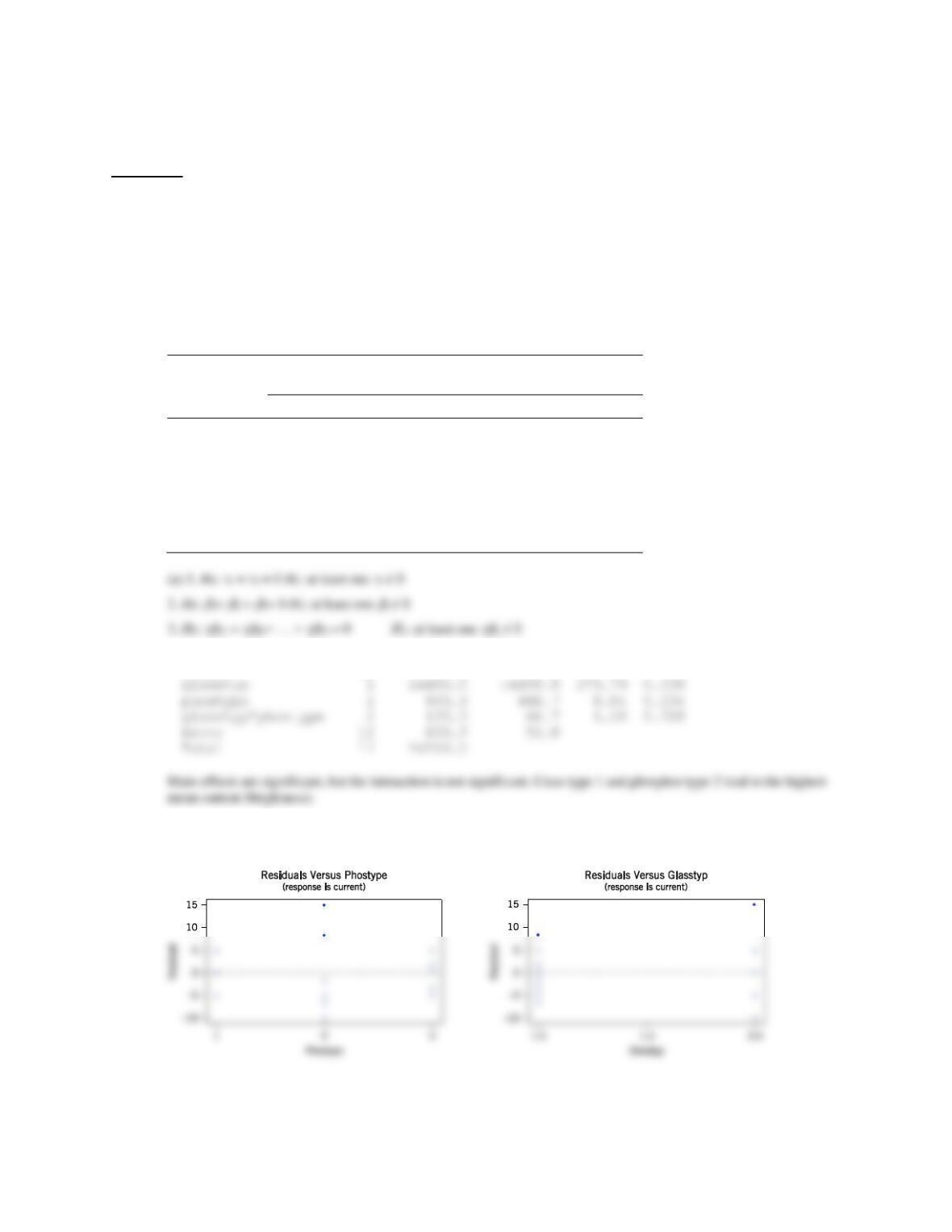
(c) Analyze the residuals from this experiment.
Glass
Type
Phosphor Type
1
2
3
1
280
300
290
290
310
285
285
295
290
2
230
260
220
235
240
225
240
235
230
(b) Analysis of Variance for current
Source DF SS MS F P
(c) There appears to be more slight variability at phosphor type 2 and glass type 2. The normal plot of the residuals
indicates that the assumption of normality is reasonable.
Applied Statistics and Probability for Engineers, 7th edition 2017
14-2
14.3.2 An engineer suspects that the surface finish of metal parts is influenced by the type of paint used and the drying time.
He selected three drying times—20, 25, and 30 minutes—and used two types of paint. Three parts are tested with each
combination of paint type and drying time. The data are as follows:
Drying Time (min)
Paint
20
25
30
1
74
73
78
64
61
85
50
44
92
2
92
98
66
86
73
45
68
88
85
(a) State the hypotheses of interest in this experiment.
(b) Test the hypotheses in part (a) and draw conclusions using the analysis of variance with
= 0.05.
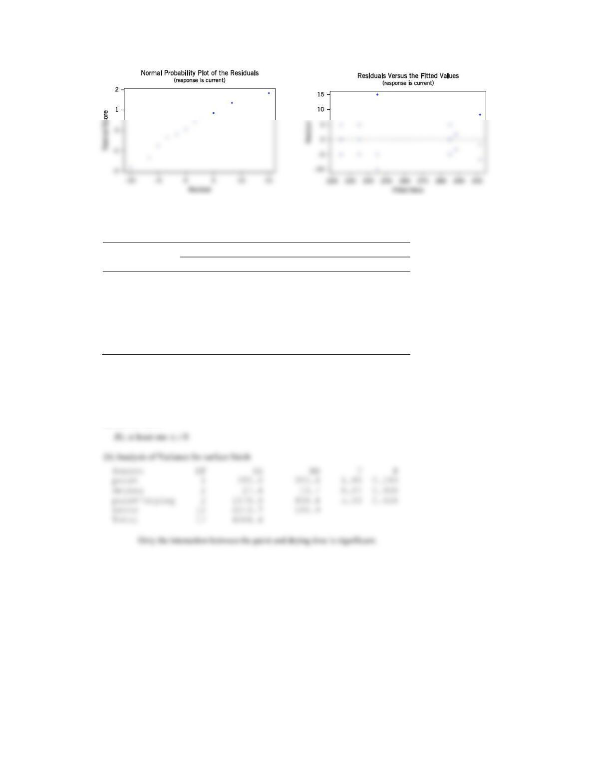
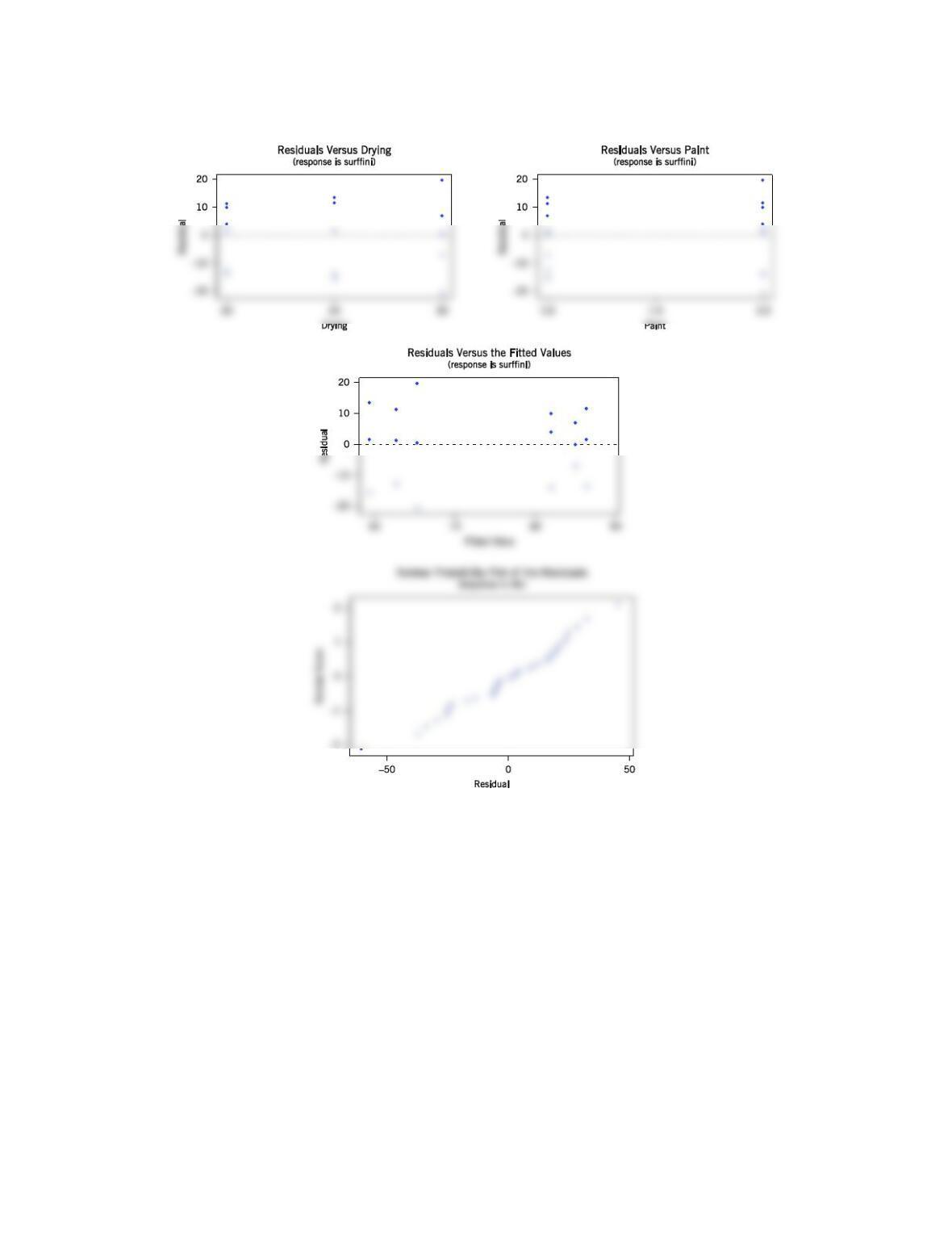
(c) Analyze the residuals from this experiment.
(a) H0:
1=
2= 0
Applied Statistics and Probability for Engineers, 7th edition 2017
14-3
(c) The residual plots appear reasonable.
14.3.3 An article in Technometrics [“Exact Analysis of Means with Unequal Variances” (2002, Vol. 44, pp. 152–160)]
described the technique of the analysis of means (ANOM) and presented the results of an experiment on insulation.
Four insulation types were tested at three different temperatures. The data are as follows:
(a) Write a model for this experiment.
(b) Test the appropriate hypotheses and draw conclusions using the analysis of variance with
= 0.05.
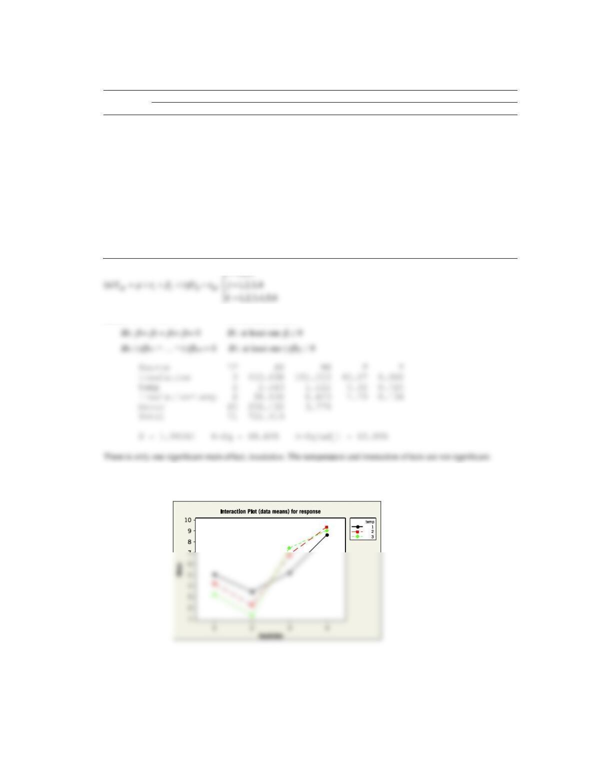
(c) Graphically analyze the interaction.
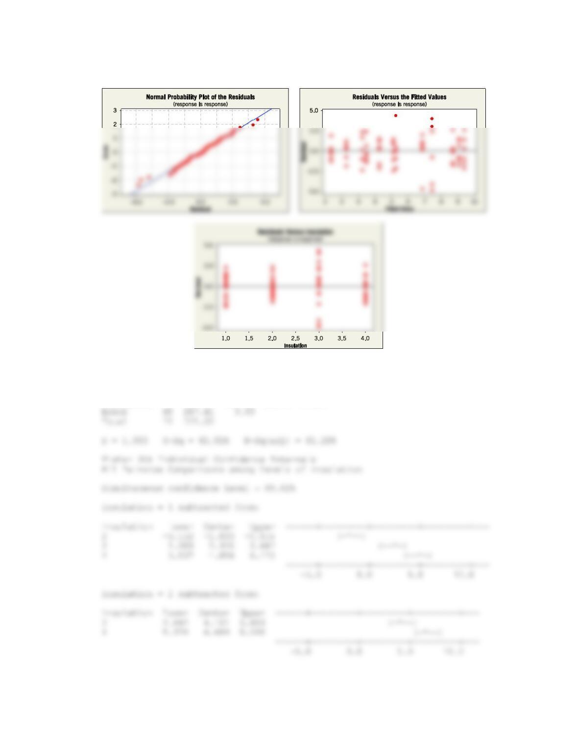
(d) Analyze the residuals from the experiment.
Applied Statistics and Probability for Engineers, 7th edition 2017
14-4
(e) Use Fisher’s LSD method to investigate the differences between mean effects of insulation type. Use
=0.05.
Insulation
Temperature (°F)
1
2
3
6.6
4
4.5
2.2
2.3
0.9
2.7
6.2
5.5
2.7
5.6
4.9
1
6
5
4.8
5.8
2.2
3.4
3
3.2
3
1.5
1.3
3.3
2.1
4.1
2.5
2.6
0.5
1.1
2
5.9
2.5
0.4
3.5
1.7
0.1
5.7
4.4
8.9
7.7
2.6
9.9
3.2
3.2
7
7.3
11.5
10.5
3
5.3
9.7
8
2.2
3.4
6.7
7
8.9
12
9.7
8.3
8
7.3
9
8.5
10.8
10.4
9.7
4
8.6
11.3
7.9
7.3
10.6
7.4
=
1,2,3
i
(b) H0:
1=
2 =
3= 0 H1: at least one
j ≠ 0
(c) Although there is some crossing of the lines, the interaction effect is minimal and was not found to be statistically
significant in part (b).
Applied Statistics and Probability for Engineers, 7th edition 2017
14-5
(d) There is more variability for insulation type 3. The normality assumption is reasonable.
(e) Here, because only one of the main effects was significant, a model which included only insulation type was fit and
LSD comparisons are made from that model:
Source DF SS MS F P
insulation 3 453.61 151.20 38.45 0.000
Applied Statistics and Probability for Engineers, 7th edition 2017
14-6
14.3.4 An experiment was conducted to determine whether either firing temperature or furnace position affects the baked
density of a carbon anode. The data are as follows:
Position
Temperature (°C)
800
825
850
1
570
1063
565
565
1080
510
583
1043
590
2
528
988
526
547
1026
538
521
1004
532
(a) State the hypotheses of interest.
(b) Test the hypotheses in part (a) using the analysis of variance with
= 0.05. What are your conclusions?
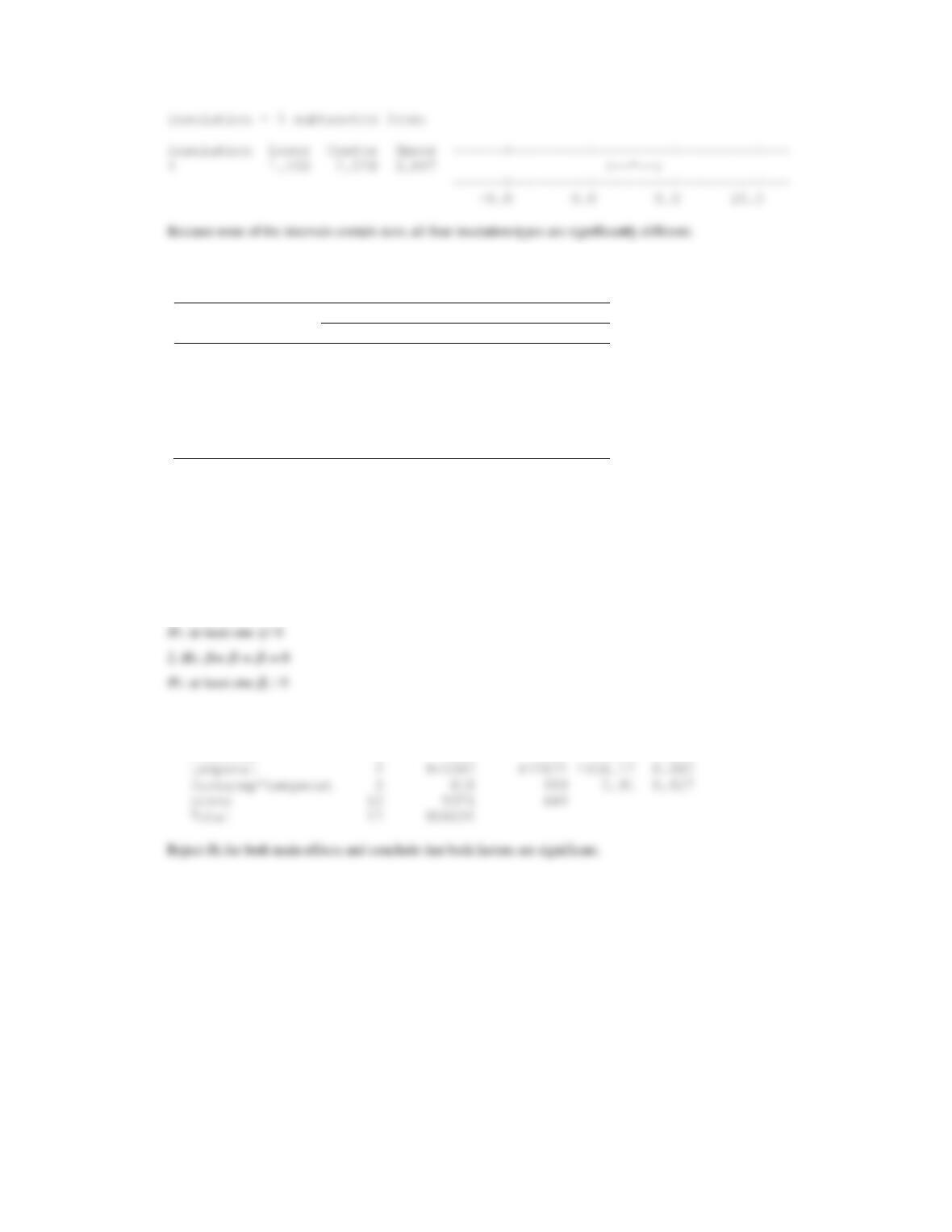
(c) Analyze the residuals from this experiment.
(d) Using Fisher’s LSD method, investigate the differences between the mean baked anode density at the three different
levels of temperature. Use
= 0.05.
(a) 1. H0:
1=
2 = 0
(b) Analysis of Variance for density
Source DF SS MS F P
furnacep 1 7160 7160 16.00 0.002
Applied Statistics and Probability for Engineers, 7th edition 2017
14-7
(c) There appears to be more variability at position 1 and at the highest temperature level. There are two unusual points
in the data.
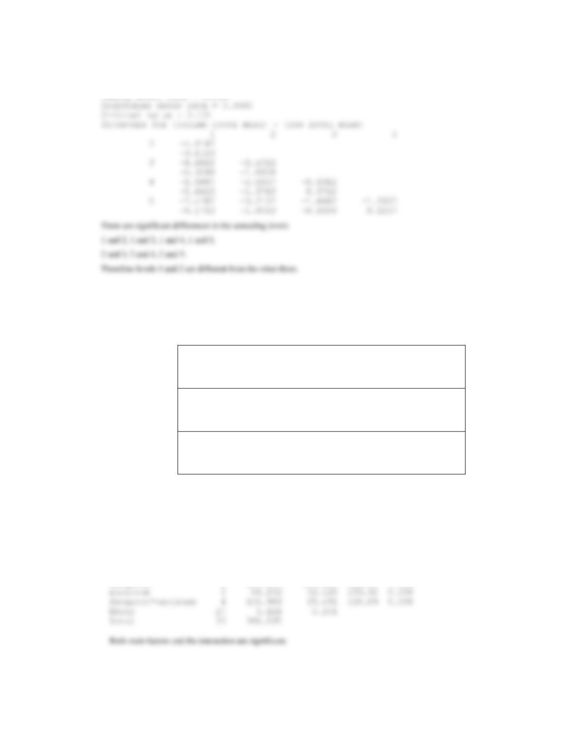
(d) Fisher’s pairwise comparisons
Family error rate = 0.117
14.3.5 An article in the IEEE Transactions on Electron Devices (November 1986, p. 1754) described a study on the effects of
two variables—polysilicon doping and anneal conditions(time and temperature)—on the base current of a bipolar
transistor. The data from this experiment follow.
(a) Is there any evidence to support the claim that either polysilicon doping level or anneal conditions affect base
current? Do these variables interact? Use
= 0.05.
(b) Graphically analyze the interaction.
(c) Analyze the residuals from this experiment.
(d) Use Fisher’s LSD method to isolate the effects of anneal conditions on base current, with
= 0.05.
Anneal (temperature/time)
900
900
950
1000
1000
60
180
60
15
30
Polysilicon doping
1 × 10²⁰
4.40
8.30
10.15
10.29
11.01
4.60
8.90
10.20
10.30
10.58
2 × 10²⁰
3.20
7.81
9.38
10.19
10.81
3.50
7.75
10.02
10.10
10.60
Applied Statistics and Probability for Engineers, 7th edition 2017
14-8
(a) Analysis of Variance for current
Source DF SS MS F P
doping 1 1.442 1.442 25.23 0.000
Applied Statistics and Probability for Engineers, 7th edition 2017
14-9
(d)
Fisher’s pairwise comparisons
Family error rate = 0.258
14.3.6 An article in the Journal of Testing and Evaluation (1988, Vol. 16, pp. 508–515) investigated the effects of cyclic
loading frequency and environment conditions on fatigue crack growth at a constant 22 MPa stress for a particular
material. The data follow. The response variable is fatigue crack growth rate.
Environment
Air
H2O
Salt H2O
10
2.29
2.06
1.90
2.47
2.05
1.93
2.48
2.23
1.75
2.12
2.03
2.06
Frequency
1
2.65
3.20
3.10
2.68
3.18
3.24
2.06
3.96
3.98
2.38
3.64
3.24
0.1
2.24
11.00
9.96
2.71
11.00
10.01
2.81
9.06
9.36
2.08
11.30
10.40
(a) Is there indication that either factor affects crack growth rate? Is there any indication of interaction?
Use
= 0.05.
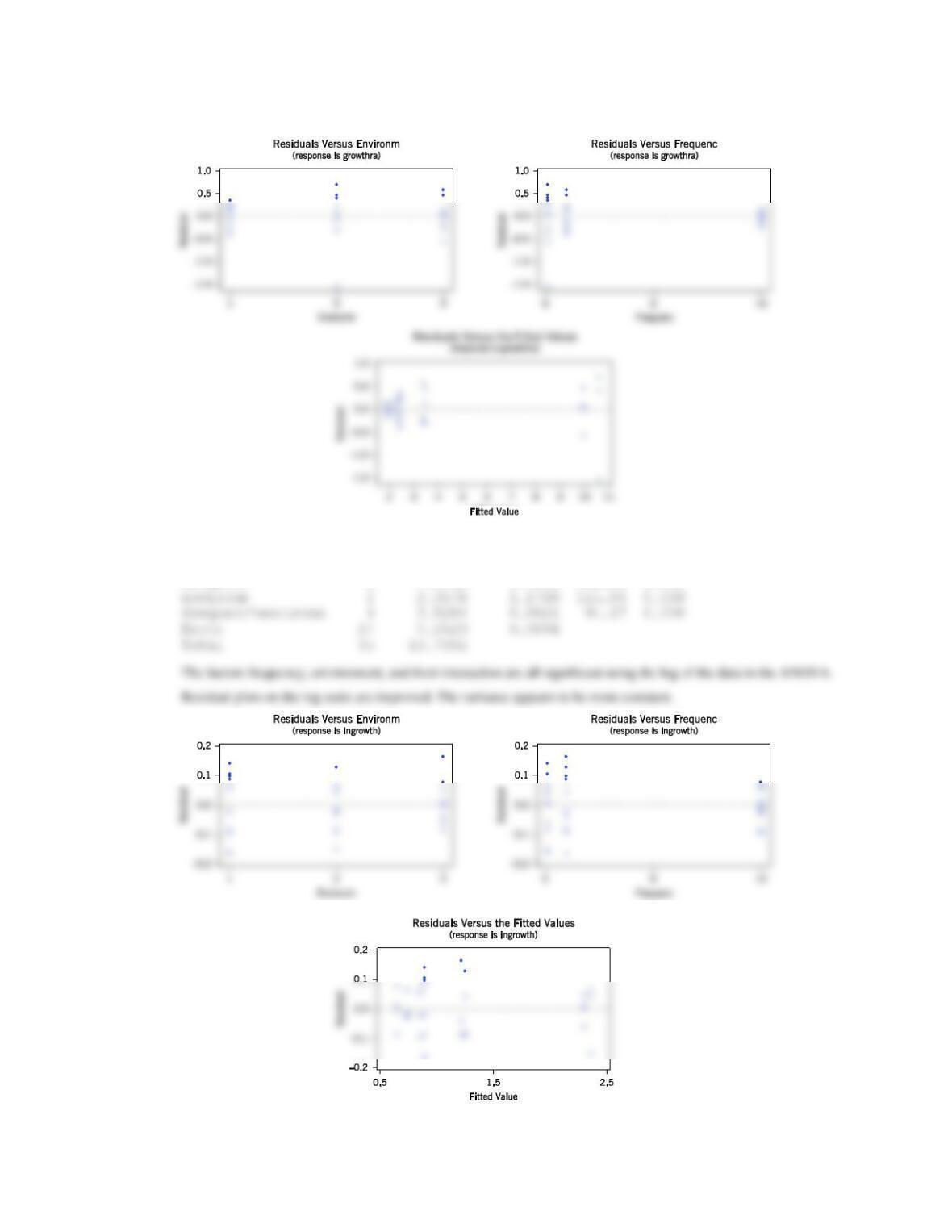
(b) Analyze the residuals from this experiment.
(c) Repeat the analysis in part (a) using ln(y) as the response. Analyze the residuals from this new response variable and
comment on the results.
(a) Analysis of Variance for crack growth
Source DF SS MS F P
frequenc 2 209.893 104.946 522.40 0.000
Applied Statistics and Probability for Engineers, 7th edition 2017
14-10
(b) There appear to be some problems with constant variance in the residual plots.
(c) Analysis of Variance of Ln(Crack Growth)
Source DF SS MS F P
frequenc 2 7.5702 3.7851 404.09 0.000
Applied Statistics and Probability for Engineers, 7th edition 2017
14-11
14.3.7 An article in Bioresource Technology [“Quantitative Response of Cell Growth and Tuber Polysaccharides Biosynthesis
by Medicinal Mushroom Chinese Truffle Tuber Sinense to Metal Ion in Culture Medium” (2008, Vol. 99(16), pp.
7606–7615)] described an experiment to investigate the effect of metal ion concentration to the production of
extracellular polysaccharides (EPS). It is suspected that Mg2+ and K+ (in mill molars) are related to EPS. The data from
a full factorial design follow.
(a) State the hypotheses of interest.
(b) Test the hypotheses with
= 0.5.
(c) Analyze the residuals and plot residuals versus the predicted production.
Run
Mg2+ (mM)
K+ (mM)
EPS (g/L)
1
40
5
3.88
2
50
15
4.23
3
40
10
4.67
4
30
5
5.86
5
50
10
4.50
6
50
5
3.62
7
30
15
3.84
8
40
15
3.25
9
30
10
4.18
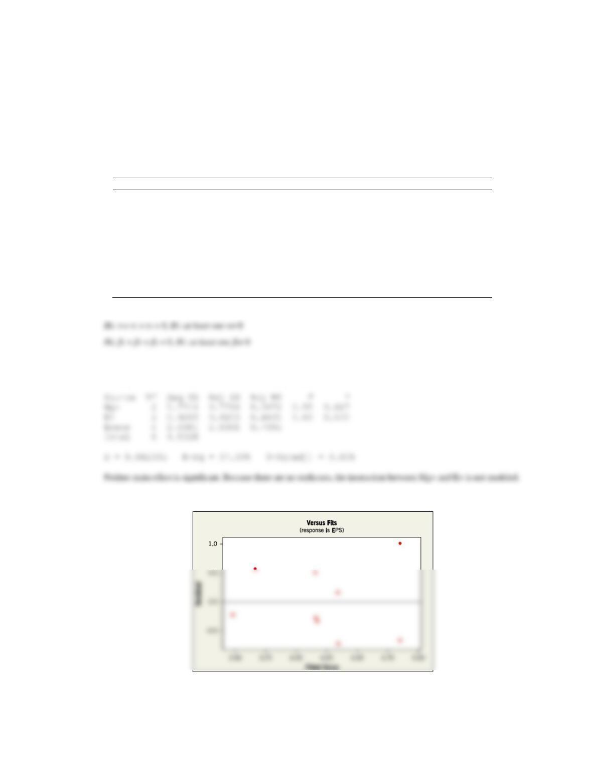
(a)
(b)
Analysis of Variance for EPS, using Adjusted SS for Tests
(c) From the residuals versus fitted values plot, no departures from assumptions are evident.
Applied Statistics and Probability for Engineers, 7th edition 2017
14-12
Section 14.4
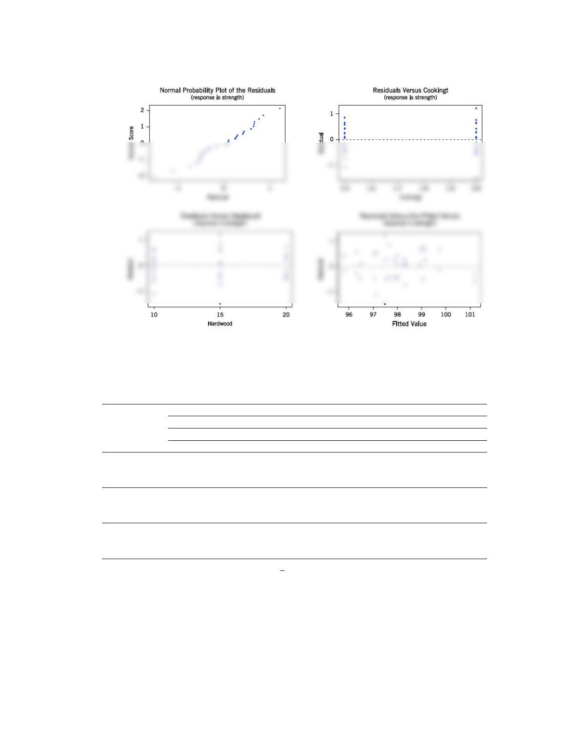
14.4.1 The percentage of hardwood concentration in raw pulp, the freeness, and the cooking time of the pulp are being
investigated for their effects on the strength of paper. The data from a three-factor factorial experiment are shown in the
following table.
(a) Analyze the data using the analysis of variance assuming that all factors are fixed. Use
= 0.05.
(b) Compute approximate P-values for the F-ratios in part (a).
(c) The residuals are found from
=−
ijkl ijkl ijk
e y y
. Graphically analyze the residuals from this experiment.
Hardwood
Concentration %
Cooking Time 1.5 hours
Cooking Time 2.0 hours
Freeness
Freeness
350
500
650
350
500
650
96.6
97.7
99.4
98.4
99.6
100.6
10
96.0
96.0
99.8
98.6
100.4
100.9
98.5
96.0
98.4
97.5
98.7
99.6
15
97.2
96.9
97.6
98.1
96.0
99.0
97.5
95.6
97.4
97.6
97.0
98.5
20
96.6
96.2
98.1
98.4
97.8
99.8
Parts (a) and (b)
Analysis of Variance for strength
Source DF SS MS F P
Applied Statistics and Probability for Engineers, 7th edition 2017
14-13
(c) The residual plots do not indicate serious problems with normality or equality of variance.
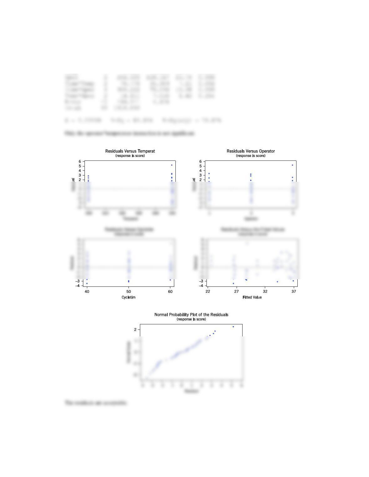
14.4.2 The quality control department of a fabric finishing plant is studying the effects of several factors on dyeing for a blended
cotton/synthetic cloth used to manufacture shirts. Three operators, three cycle times, and two temperatures were selected,
and three small specimens of cloth were dyed under each set of conditions. The finished cloth was compared to a standard,
and a numerical score was assigned. The results are shown in the following table.
(a) State and test the appropriate hypotheses using the analysis of variance with α = 0.05.
Temperature
300°
350°
Operator
Operator
Cycle Time
1
2
3
1
2
3
23
27
31
24
38
34
40
24
28
32
23
36
36
25
26
28
28
35
39
36
34
33
37
34
34
50
35
38
34
39
38
36
36
39
35
35
36
31
28
35
26
26
36
28
60
24
35
27
29
37
26
27
34
25
25
34
34
(b) The residuals may be obtained from
=−
ijkl ijkl ijk
e y y
. Graphically analyze the residuals from this experiment.
Applied Statistics and Probability for Engineers, 7th edition 2017
14-14
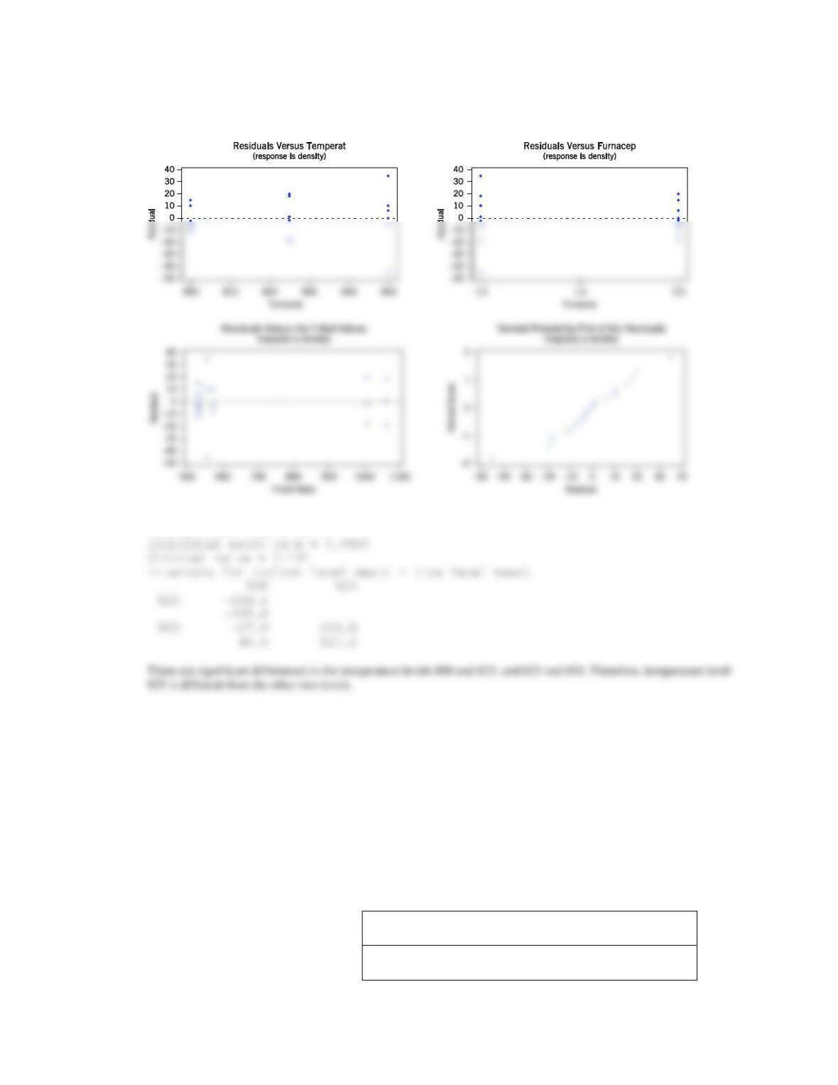
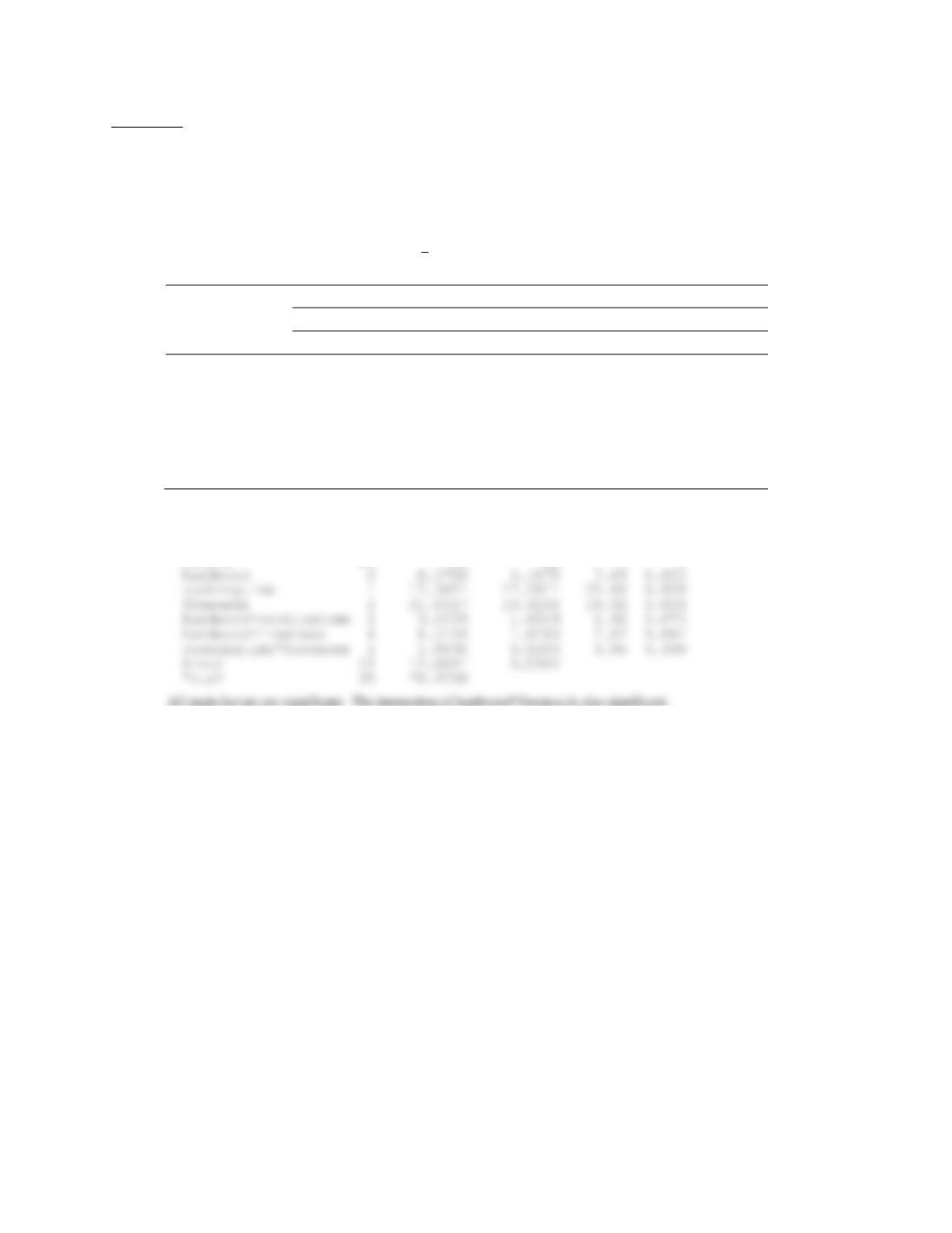
(a) Analysis of Variance for dying score, using Adjusted SS for Tests
Source DF SS MS F P
Time 2 396.778 198.389 39.85 0.000
Temp 1 73.500 73.500 14.77 0.000
(b)

Applied Statistics and Probability for Engineers, 7th edition 2017
Section 14.5
14.5.1 Four factors are thought to influence the taste of a soft-drink beverage: type of sweetener (A), ratio of syrup to
water (B), carbonation level (C), and temperature (D). Each factor can be run at two levels, producing a 24 design. At
each run in the design, samples of the beverage are given to a test panel consisting of 20 people. Each tester assigns the
beverage a point score from 1 to 10. Total score is the response variable, and the objective is to find a formulation that
maximizes total score. Two replicates of this design are run, and the results are shown in the table. Analyze the data
and draw conclusions. Use a = 0.05 in the statistical tests.
Treatment
Combination
Replicate
I
II
(1)
159
163
a
168
175
b
158
163
ab
166
168
c
175
178
ac
179
183
bc
173
168
abc
179
182
d
164
159
ad
187
189
bd
163
159
abd
185
191
cd
168
174
acd
197
199
bcd
170
174
abcd
194
198
Term Effect Coef SE Coef T P
Constant 175.250 0.5467 320.59 0.000
A 17.000 8.500 0.5467 15.55 0.000
B -1.625 -0.812 0.5467 -1.49 0.157
C 10.875 5.438 0.5467 9.95 0.000
B*D 1.250 0.625 0.5467 1.14 0.270
C*D -1.250 -0.625 0.5467 -1.14 0.270
A*B*C 0.750 0.375 0.5467 0.69 0.503
14-16
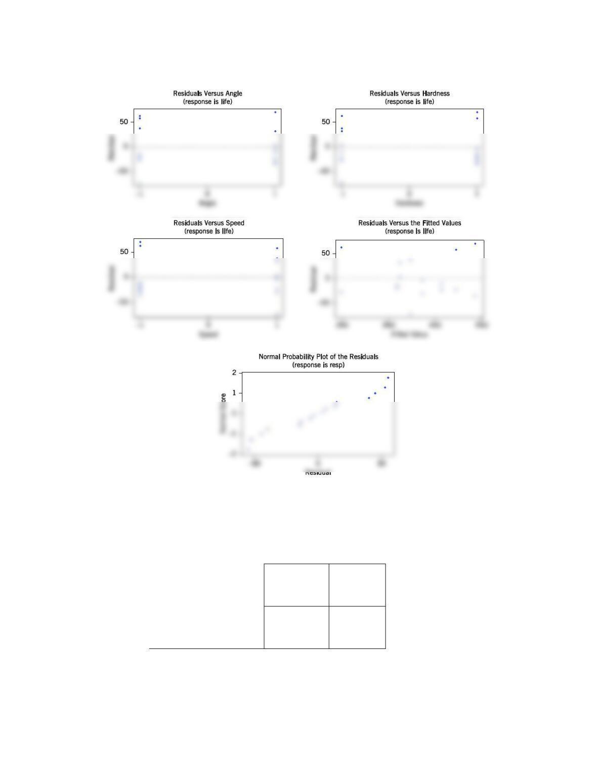
14.5.2 An engineer is interested in the effect of cutting speed (A), metal hardness (B), and cutting angle (C) on the life of a
cutting tool. Two levels of each factor are chosen, and two replicates of a 23 factorial design are run. The tool life data
(in hours) are shown in the following table.
Treatment Combination
Replicate
I
II
(1)
221
311
a
325
435
b
354
348
ab
552
472
c
440
453
ac
406
377
bc
605
500
abc
392
419
(a) Analyze the data from this experiment.
(b) Find an appropriate regression model that explains tool life in terms of the variables used in the experiment.
(c) Analyze the residuals from this experiment.
(a) Analysis of Variance for life (coded units)
Source DF SS MS F P
A 1 1332 1332 0.54 0.483
B 1 28392 28392 11.53 0.009
(b) Estimated Effects and Coefficients for life (coded units)
Term Effect Coef SE Coef T P
Constant 413.13 12.41 33.30 0.000
speed 18.25 9.12 12.41 0.74 0.483
Applied Statistics and Probability for Engineers, 7th edition 2017
14-17
(c) Analysis of the residuals shows that all assumptions are reasonable.
14.5.3 An article in IEEE Transactions on Semiconductor Manufacturing (1992, Vol. 5, pp. 214–222) described an
experiment to investigate the surface charge on a silicon wafer. The factors thought to influence induced surface charge
are cleaning method (spin rinse dry or SRD and spin dry or SD) and the position on the wafer where the charge was
measured. The surface charge (×1011 q/cm3) response data follow:
Test Position
L
R
SD
1.66
1.84
1.90
1.84
Cleaning Method
1.92
1.62
SRD
−4.21
−7.58
−1.35
−2.20
−2.08
−5.36
(a) Estimate the factor effects.
(b) Which factors appear important? Use
= 0.05.
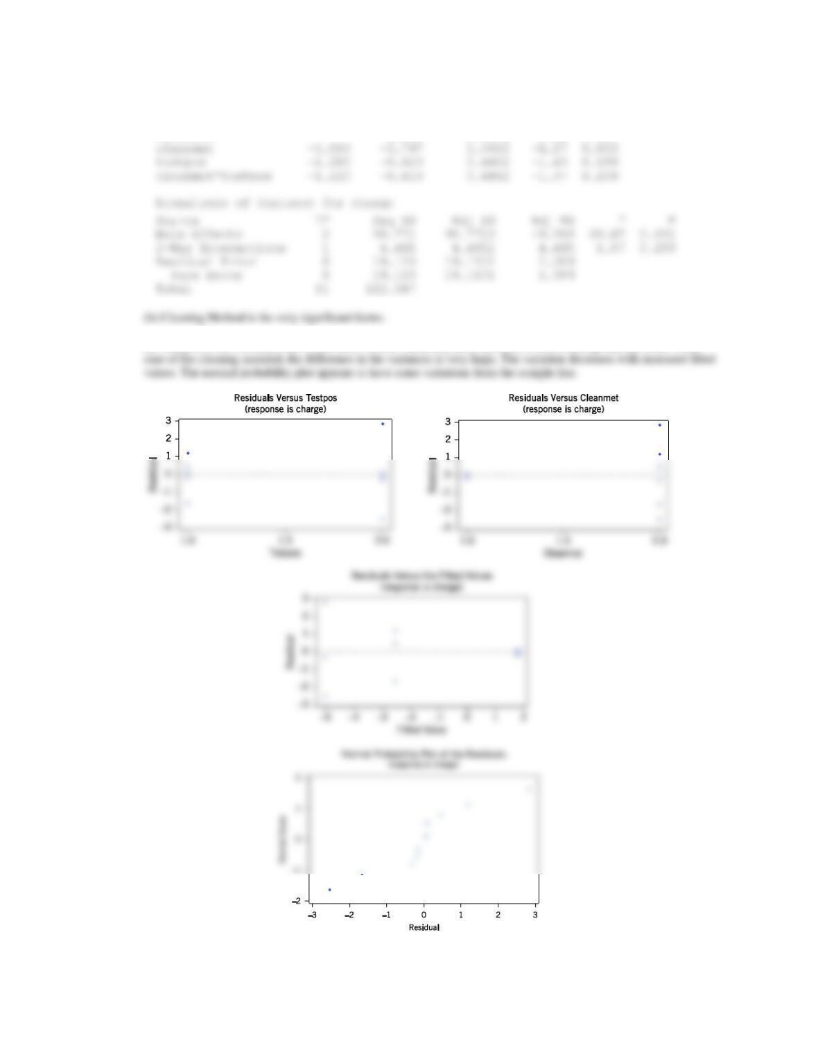
(c) Analyze the residuals from this experiment.
Applied Statistics and Probability for Engineers, 7th edition 2017
14-18
(a) Estimated Effects and Coefficients for charge
Term Effect Coef StDev Coef T P
Constant -1.000 0.4462 -2.24 0.055
(c) Analysis of the residuals shows that there is more variability at test position R and cleaning material SRD. In the

Applied Statistics and Probability for Engineers, 7th edition 2017
14-19
14.5.4 An article in Talanta (2005, Vol. 65, pp. 895–899) presented a 23 factorial design to find lead level by using flame
atomic absorption spectrometry (FAAS). The data are in the following table.
Factors
Lead Recovery (%)
Run
ST
pH
RC
R1
R2
1
−
−
−
39.8
42.1
2
+
−
−
51.3
48
3
−
+
−
57.9
58.1
4
+
+
−
78.9
85.9
5
−
−
+
78.9
84.2
6
+
−
+
84.2
84.2
7
−
+
+
94.4
90.9
8
+
+
+
94.7
105.3
The factors and levels are in the following table.
Factor
Low (−)
High (+)
Reagent concentration (RC) (mol 1−1)
5 × 10⁻⁶
5 × 10⁻⁵
pH
6.0
8.0
Shaking time (ST) (min)
10
30
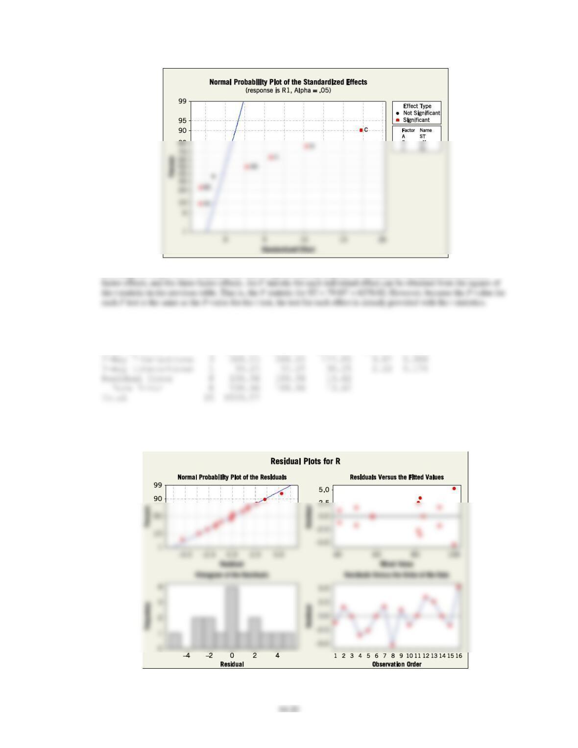
(a) Construct a normal probability plot of the effect estimates. Which effects appear to be large?
(b) Conduct an analysis of variance to confirm your findings for part (a).
(c) Analyze the residuals from this experiment. Are there any problems with model adequacy?
Factorial Fit: R1 Versus ST, pH, RC
Estimated Effects and Coefficients for R1 (coded units)
Term Effect Coef SE Coef T P
Constant 73.675 0.9226 79.85 0.000
ST 10.775 5.387 0.9226 5.84 0.000
Applied Statistics and Probability for Engineers, 7th edition 2017
(b) Computer output below combines the sum of squares and the degrees of freedom for the main effects, the two-
Analysis of Variance for R1 (coded units)
Source DF Seq SS Adj SS Adj MS F P
Main Effects 3 5992.81 5992.81 1997.60 146.67 0.000
(c) The normality assumption is reasonable. The plot of residuals versus the predicted values indicates some greater
variability for larger fitted values so that some departure from assumptions is indicated. The actual time order of the
observations was not provided so the plot versus observation order is not relevant.