15
65
0.12
0.75
0
2−
0
1.153
16
65
0.5
0.75
0
2
0
6.333
17
65
0.25
0.42
0
0
2−
2.533
18
65
0.25
1.33
0
0
2
3.2
19
28
0.25
0.75
2−
0
0
3.233
20
150
0.25
0.75
2
0
0
2.967
21
65
0.12
0.75
0
2−
0
1.21
22
65
0.5
0.75
0
2
0
6.733
23
65
0.25
0.42
0
0
2−
2.833
24
65
0.25
1.33
0
0
2
3.267
Levels
Lowest
Low
Center
High
Highest
Coding
2−
-1
0
1
2
Speed, V (m/min)
28
36
65
117
150
Feed, f (mm/rev)
0.12
0.15
0.25
0.4
0.5
Depth of cut, d (mm)
0.42
0.5
0.75
1.125
1.33
(a) Fit both first- and second-order models to the data. Determine test statistics for the following
parts of models.
(b) Comment on the adequacies of these models. Which reduced model we can fit?
(c) What are the coefficients to predict surface roughness in terms of the coded units?
SOLUTION
(a), (b) First-order model:
Estimated Regression Coefficients for y (surface roughness)
Term
Coef
SE Coef
T
P
Constant
3.2422
0.112
28.955
0
2
x
1.8931
0.1371
13.804
0
Analysis of Variance for y
Source
DF
Seq SS
Adj SS
Adj MS
F
P
Regression
3
59.0253
59.0253
19.6751
65.39
0
Linear
3
59.0253
59.0253
19.6751
65.39
0
Residual Error
20
Lack-of-Fit
11
19.26
0
Pure Error
9
Total
23
65.0432
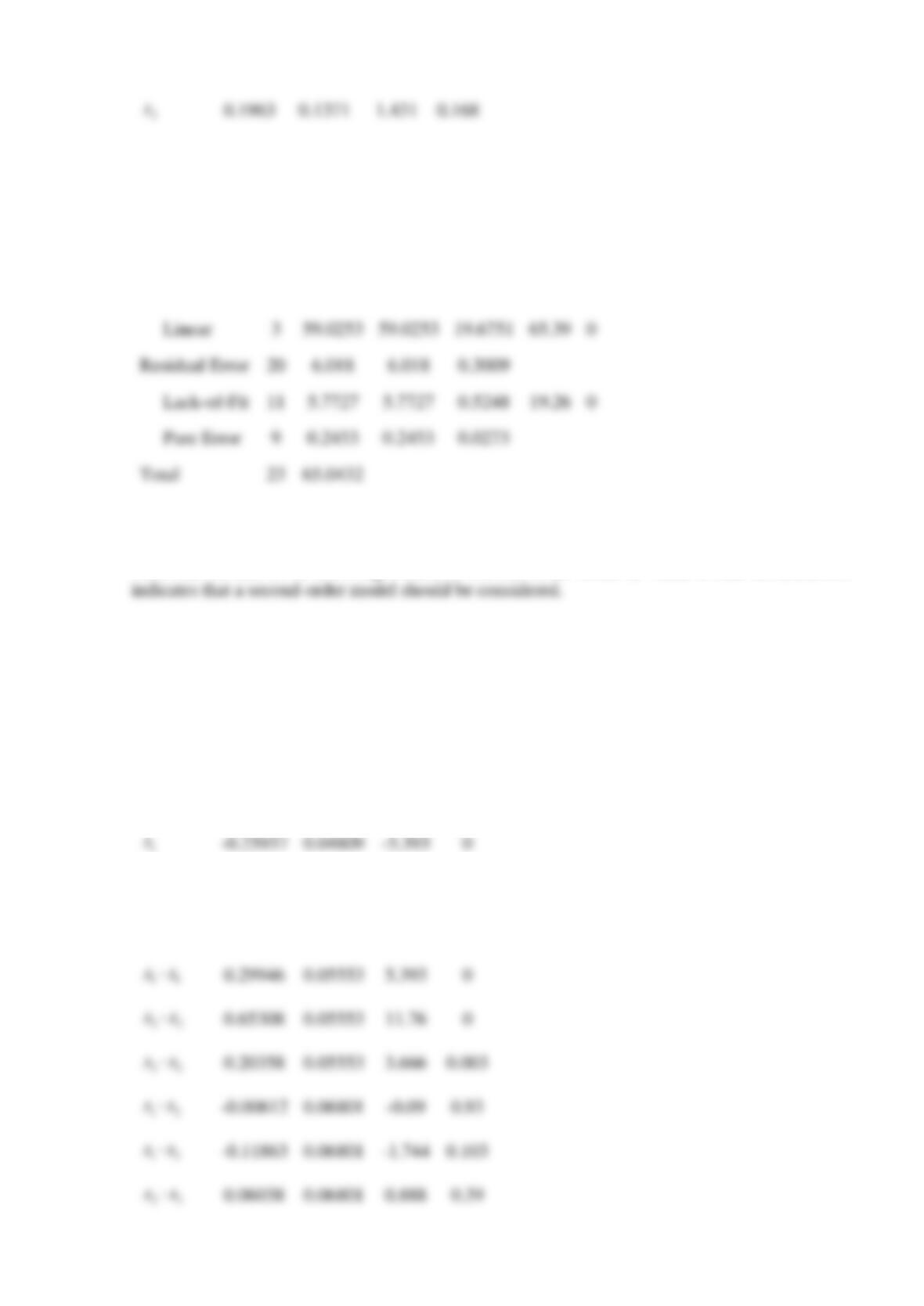
Note that the lack-of-fit test is significant for the first-order model (P-value is near zero) and this
Second-order model:
Estimated Regression Coefficients for y
Term
Coef
SE Coef
T
P
Constant
2.47142
0.0878
28.147
0
2
x
1.89296
0.04809
39.361
0
3
x
0.19625
0.04809
4.081
0.001
0.65308
0.05553
11.76
0
-0.00612
0.06801
0.93
3
x
Analysis of Variance for y
Source
DF
Seq SS
Adj SS
Adj MS
F
P
Regression
9
64.5252
64.5252
7.1695
193.74
0
Residual Error
14
0.5181
0.5181
0.037
Lack-of-Fit
5
0.2728
0.2728
0.0546
2
0.172
Pure Error
9
0.2453
0.2453
0.0273
Total
23
65.0432
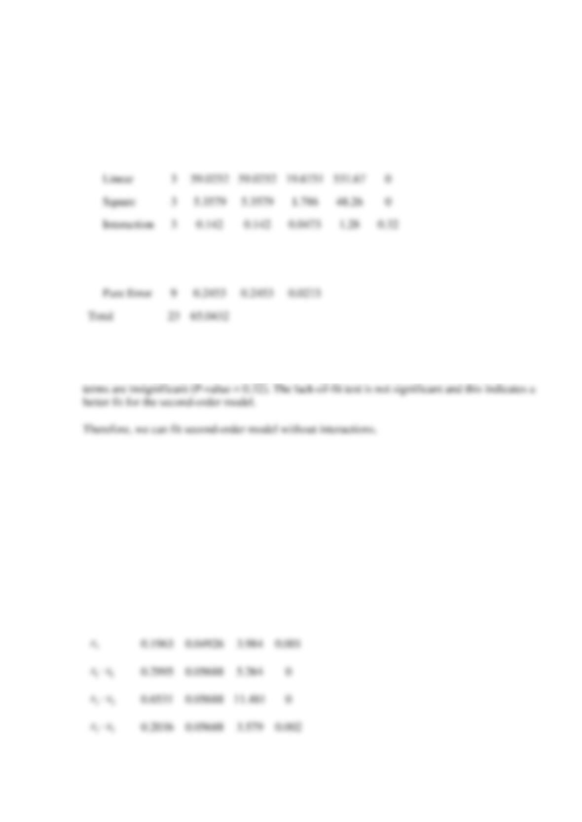
The linear and pure quadratic terms appear to be significant (P-values = 0) while the interaction
(c) Reduced model:
Estimated Regression Coefficients for y
Term
Coef
SE Coef
T
P
Constant
2.4714
0.08994
27.478
0
1
x
-0.2594
0.04926
-5.265
0
2
x
1.8930
0.04926
38.425
0
0.04926
0.001
0.05688
0
0.05688
11.481
0
Linear
3
59.0252
59.0252
19.6751
531.67
0
Square
3
5.3579
5.3579
1.786
48.26
0
Interaction
3
0.142
0.142
0.0473
1.28
0.32
Reserve Problems Chapter 14 Section 11 Problem 5
Effects of probe and target concentration and particle number in immobilization and
hybridization on a microparticle-based DNA hybridization assay are investigated. Mean
fluorescence is the response. Particle concentration was transformed to surface area
measurements. Other concentrations were measured in micromoles per liter (μM). Data follow.
Run
Immobilization
area
(cm2)
Probe
area
(μM)
Hybridization
(cm2)
Target
(μM)
Mean
Fluorescence
1
0.35
0.025
0.35
0.025
4.7
2
7
0.025
0.35
0.025
4.7
3
0.35
2.5
0.35
0.025
28
4
7
2.5
0.35
0.025
81.2
5
0.35
0.025
3.5
0.025
5.7
6
7
0.025
3.5
0.025
4
7
0.35
2.5
3.5
0.025
12.2
8
7
2.5
3.5
0.025
19.5
9
0.35
0.025
0.35
5
4.4
10
7
0.025
0.35
5
2.6
11
0.35
2.5
0.35
5
83.7
12
7
2.5
0.35
5
85.2
13
0.35
0.025
3.5
5
6.8
14
7
0.025
3.5
5
2.4
15
0.35
2.5
3.5
5
76
16
7
2.5
3.5
5
77.9
17
0.35
5
2
2.5
42.6
18
7
5
2
2.5
52.3
19
3.5
0.025
2
2.5
2.6
20
3.5
2.5
2
2.5
72.8
21
3.5
5
0.35
2.5
47
22
3.5
5
3.5
2.5
54.4
23
3.5
5
2
0.025
30.8

24
3.5
5
2
5
64.8
25
3.5
5
2
2.5
51.6
26
3.5
5
2
2.5
52.6
27
3.5
5
2
2.5
55.8
Adjust these data to fit the central composite design and suppose that the values of parameters
are following:
Run
Immobilization
area
(cm2)
Probe
area
(μM)
Hybridization
(cm2)
Target
(μM)
Mean
Fluorescence
1
0
0
0.35
0
4.7
2
7
0
0.35
0
4.7
3
0
5
0.35
0
28
4
7
5
0.35
0
81.2
5
0
0
3.5
0
5.7
6
7
0
3.5
0
4
7
0
5
3.5
0
12.2
8
7
5
3.5
0
19.5
9
0
0
0.35
5
4.4
10
7
0
0.35
5
2.6
11
0
5
0.35
5
83.7
12
7
5
0.35
5
85.2
13
0
0
3.5
5
6.8
14
7
0
3.5
5
2.4
15
0
5
3.5
5
76
16
7
5
3.5
5
77.9
17
0
2.5
1.925
2.5
42.6
18
7
2.5
1.925
2.5
52.3
19
3.5
0
1.925
2.5
2.6
20
3.5
5
1.925
2.5
72.8
21
3.5
2.5
0.35
2.5
47
22
3.5
2.5
3.5
2.5
54.4
23
3.5
2.5
1.925
0
30.8
24
3.5
2.5
1.925
5
64.8
25
3.5
2.5
1.925
2.5
51.6
26
3.5
2.5
1.925
2.5
52.6
27
3.5
2.5
1.925
2.5
55.8
(a) What type of design is used?
(b) Fit a second-order response surface model to the data.
SOLUTION
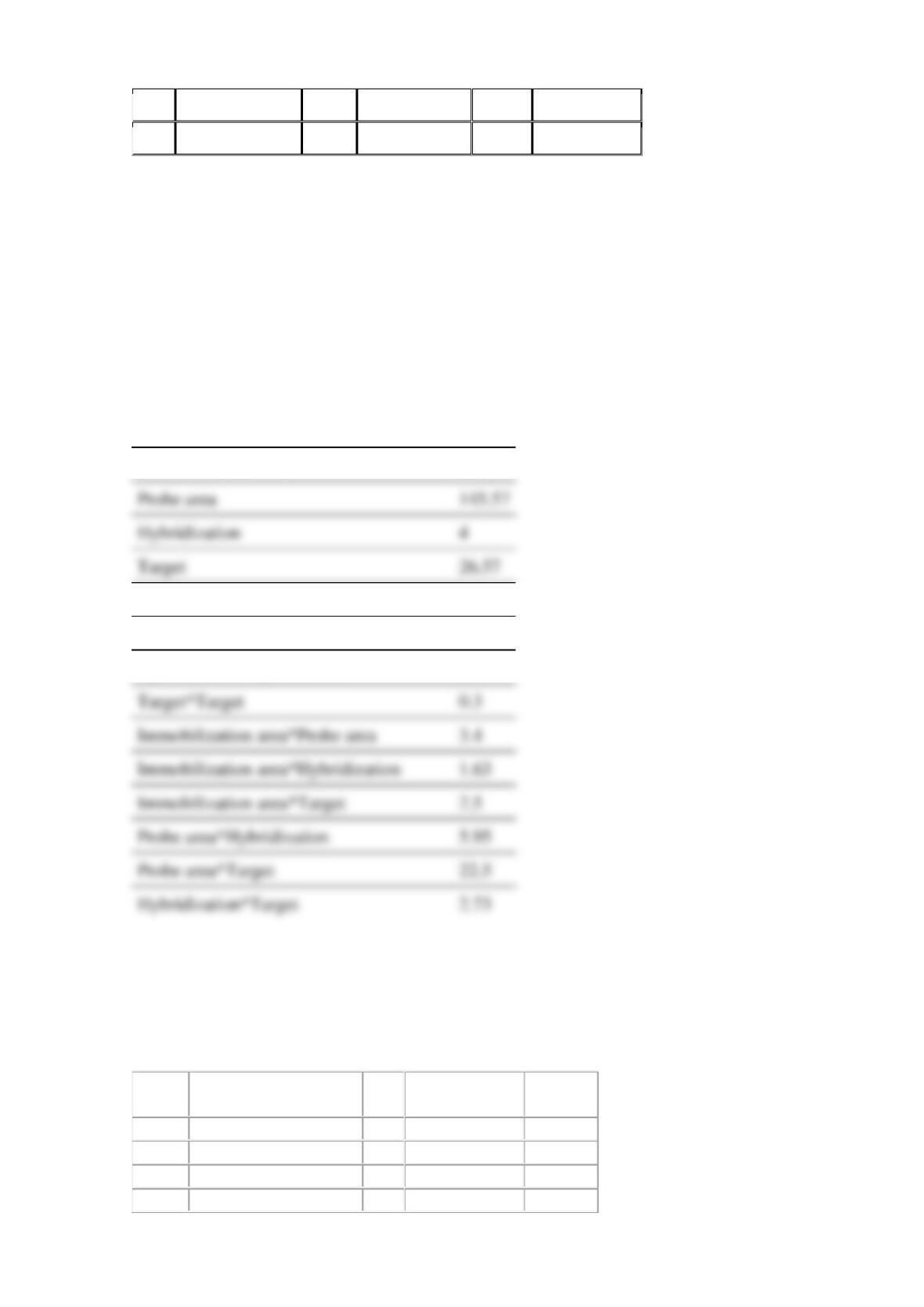
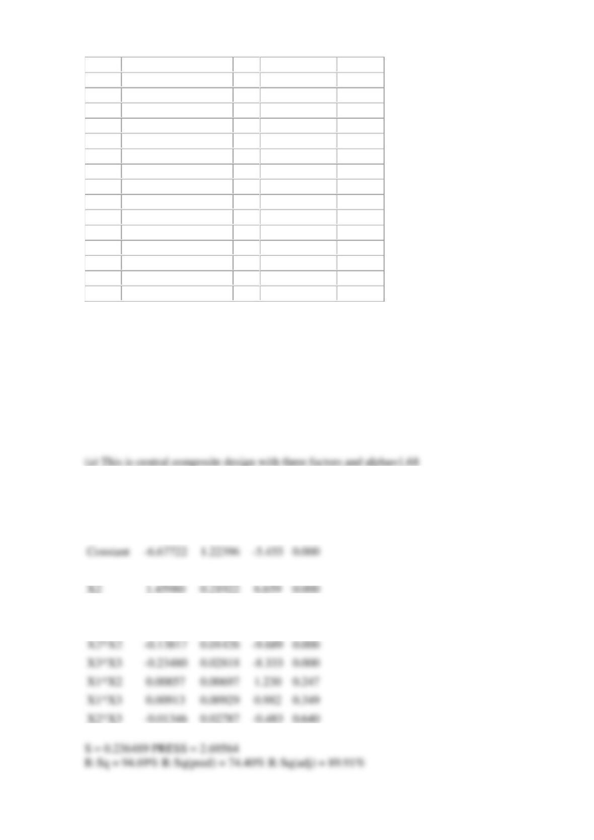
(a) It is a central composite design with four factors, three center points, and α = 1.
(b) The analysis was performed using coded units.
Analysis of Variance for Mean Fluorescence gives
Factor
F
Immobilization area
2.53
Immobilization area*Immobilization area
0.36
Probe area*Probe area
4.87
Hybridization*Hybridization
0
Target*Target
0.3
Immobilization area*Probe area
3.4
Immobilization area*Hybridization
1.63
Immobilization area*Target
2.5
Probe area*Hybridization
5.95
Probe area*Target
22.5
Hybridization*Target
2.73
Reserve Problems Chapter 14 Section 11 Problem 6
An experiment to optimize the production of polyhydroxybutyrate (PHB) is described. Inoculum
age, pH, and substrate were selected as factors, and a central composite design was conducted.
Data follow.
Run
Inoculum age
(h)
pH
Substrate
(g/L)
PHB
(g/L)
1
12
4
1
0.84
2
24
8
1
0.55
3
18
6
2.5
1.96
4
28
6
2.5
1.2
Probe area
145.57
Hybridization
4
Target
26.57
5
12
4
4
0.783
6
18
6
2.5
1.66
7
18
6
2.5
2.22
8
18
6
5
0.8
9
12
8
4
0.48
10
18
6
2.5
1.97
11
18
6
2.5
2.2
12
18
6
2.5
2.25
13
18
2
2.5
0.2
14
18
6
0
0.22
15
12
8
1
0.37
16
24
8
4
0.66
17
24
4
1
0.28
18
24
4
4
0.88
19
18
9
2.5
0.3
20
7
6
2.5
0.42
(a) What type of design is used?
(b) Fit a second-order response surface model to the data. Use uncoded units.
What is the F test statistic for test of hypothesis about main factors?
(c) What values can you recommend for inoculum age, pH, and substrate to maximize
production?
SOLUTION
(b)
The analysis was done using uncoded units.
Estimated Regression Coefficients for PHB
Term
Coef
SE_Coef
T
P
Constant
-6.67722
1.22396
-5.455
0.000
X1
0.32171
0.07543
4.265
0.002
X2
1.45980
0.21922
6.659
0.000
X3
1.17557
0.27859
4.220
0.002
X1*X1
-0.01071
0.00162
-6.610
0.000
X2*X2
-0.13817
0.01426
-9.689
0.000
X3*X3
-0.23480
0.02818
-8.333
0.000
X1*X2
0.00857
0.00697
1.230
0.247
X1*X3
0.00913
0.00929
0.982
0.349
X2*X3
-0.01346
0.02787
-0.483
0.640
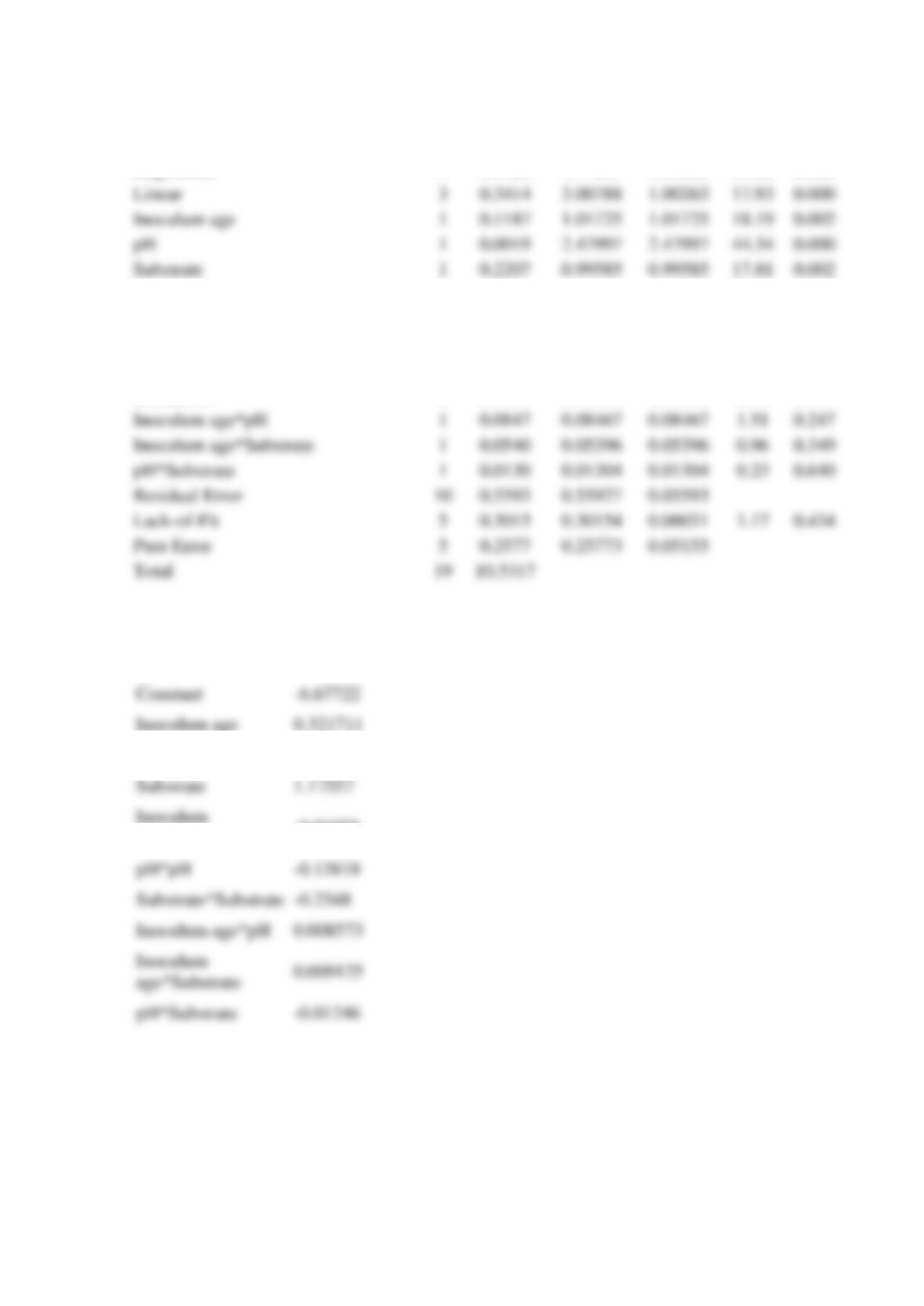
Analysis of Variance for PHB
Source
DF
Seq SS
Adj SS
Adj MS
F
P
Regression
9
9.9725
9.97247
1.10805
19.81
0.000
Square
3
9.4794
9.47940
3.15980
56.50
0.000
Inoculum age*Inoculum age
1
1.2484
2.44389
2.44389
43.70
0.000
pH*pH
1
4.3477
5.25009
5.25009
93.87
0.000
Substrate*Substrate
1
3.8832
3.88321
3.88321
69.43
0.000
Interaction
3
0.1517
0.15166
0.05055
0.90
0.473
Inoculum age*pH
1
0.0847
0.08467
0.08467
1.51
0.247
Inoculum age*Substrate
1
0.0540
0.05396
0.05396
0.96
0.349
pH*Substrate
1
0.0130
0.01304
0.01304
0.23
0.640
Residual Error
10
0.5593
0.55927
0.05593
Lack-of-Fit
5
0.3015
0.30154
0.06031
1.17
0.434
Pure Error
5
0.2577
0.25773
0.05155
Total
19
10.5317
Estimated Regression Coefficients for PHB using data in uncoded units
Term
Coef
Constant
-6.67722
Inoculum age
0.321711
pH
1.4598
Substrate
1.17557
age*Inoculum age
-0.01071
pH*pH
-0.13818
Substrate*Substrate
-0.2348
Inoculum age*pH
0.008573
age*Substrate
0.009125
pH*Substrate
-0.01346
Linear
3
0.3414
3.00788
1.00263
17.93
0.000
Inoculum age
1
0.1187
1.01725
1.01725
18.19
0.002
pH
1
0.0019
2.47997
2.47997
44.34
0.000
Substrate
1
0.2207
0.99585
0.99585
17.81
0.002
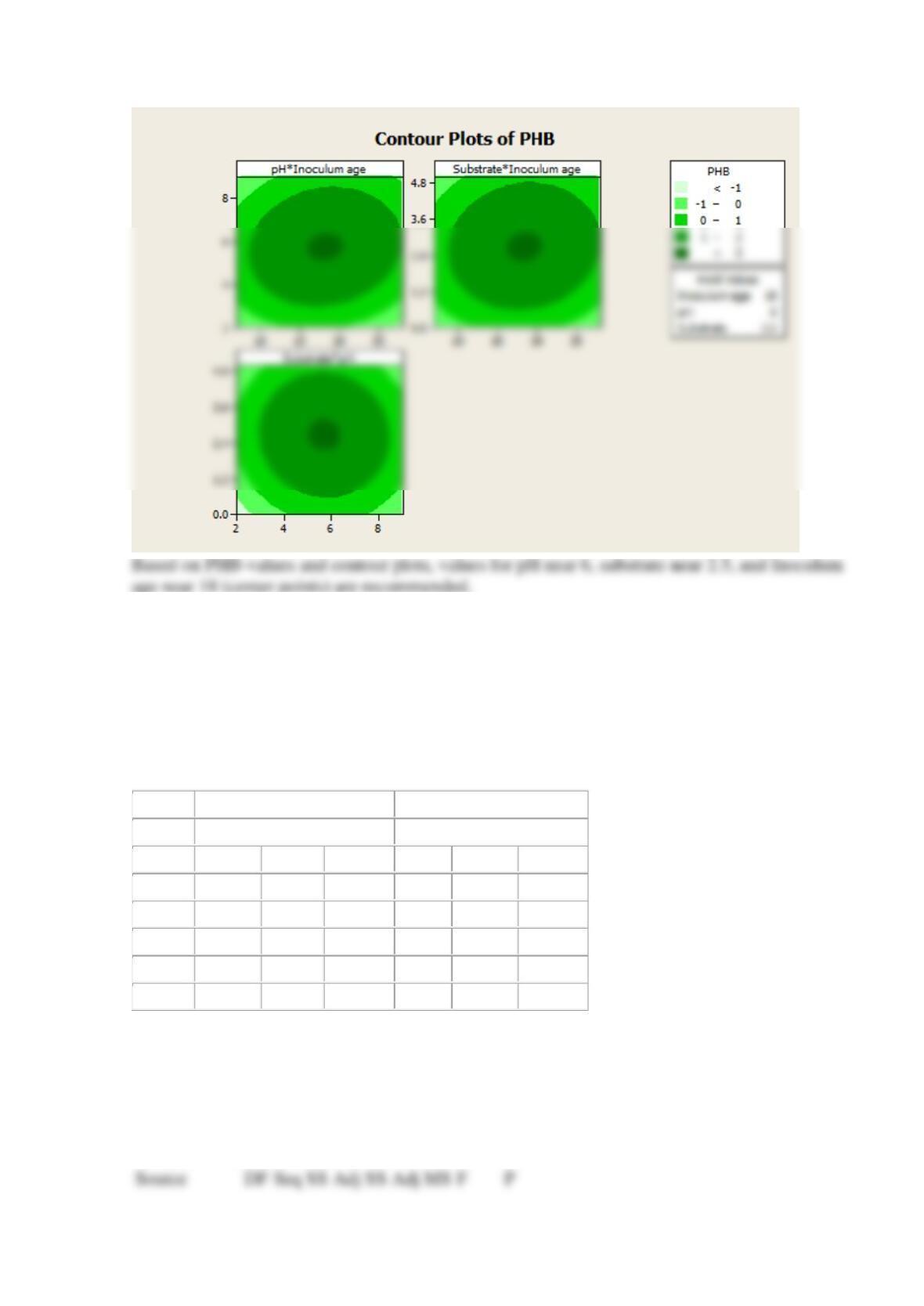
(c)
Reserve Supplemental Exercises Chapter 14 Problem 1
The time for subjects to complete tasks of different difficulty (easy, normal, difficult) on mobile
devices with different screen sizes (5″ and 7″) was considered. The five subjects are considered a
nuisance factor.
Display 5″
Display 7″
Task
Task
Subject
Easy
Normal
Difficult
Easy
Normal
Difficult
1
10.8886
0.8143
2.4379
0.9966
6.0899
0.6143
2
14.1011
1.0071
0.3810
0.6799
7.8300
1.0925
3
1.4512
0.3996
9.6069
1.5273
2.3524
6.6903
4
14.3924
3.4862
9.2766
4.9163
12.5969
6.3065
5
17.8937
2.7719
3.0259
6.9067
6.8163
8.7701
(a) State and test the appropriate hypotheses using the analysis of variance with
0.05
=
.
(b) Is the blocking variation large relative to the differences between the factor levels?
SOLUTION
(a)
Analysis of Variance for Time
Block
4
134.02
134.02
33.51
2.8
0.054
Task
2
51.49
51.49
25.75
2.15
0.142
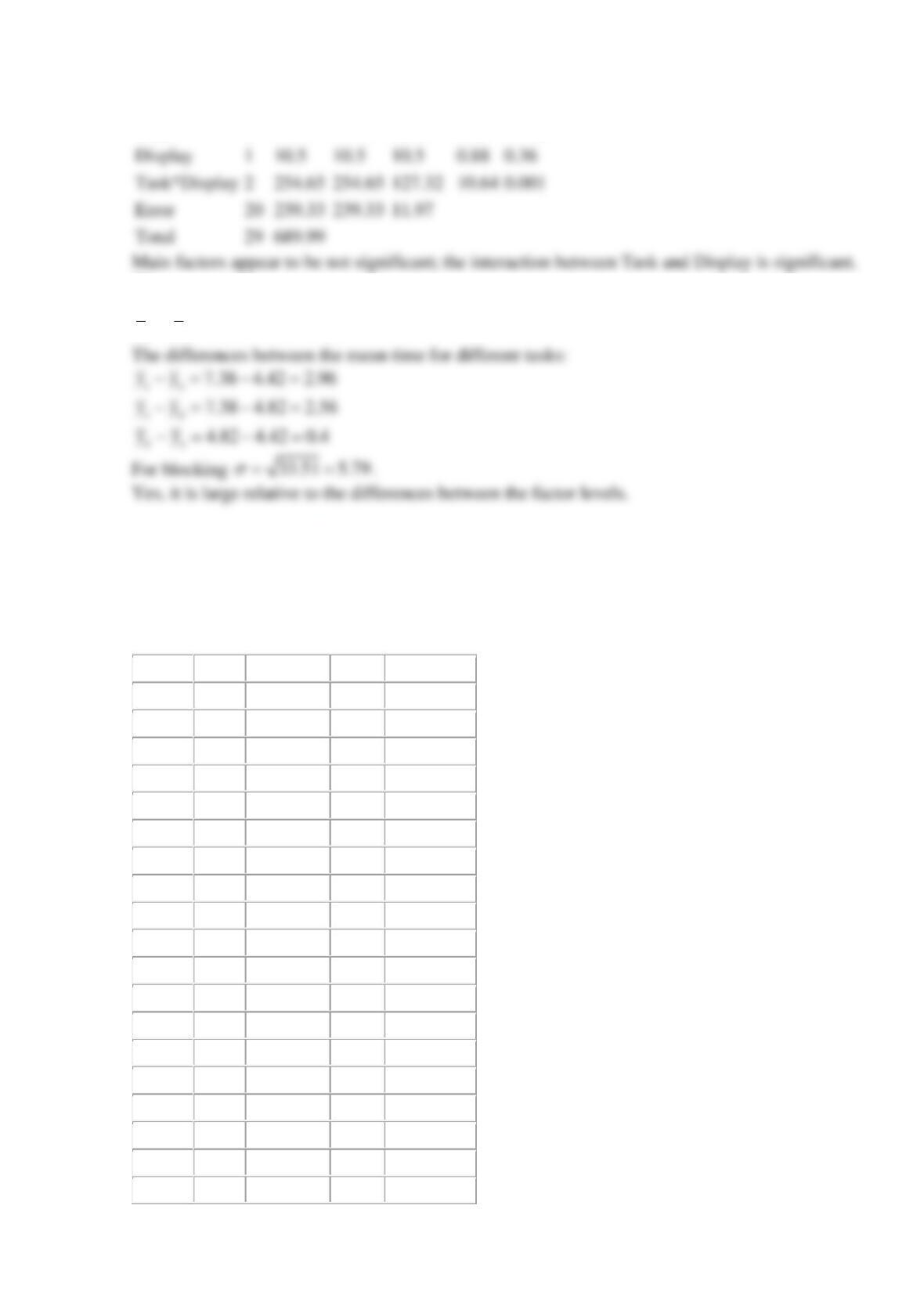
(b)
The difference between the mean time for different displays is
5″ 7” 6.13 4.95 1.18yy− = − =
Reserve Supplemental Exercises Chapter 14 Problem 2
The effect of factors on the lifting index (greater lifting index implies greater back pain) was
considered. Factors were weight (kg), twisting angle (degrees), lifting frequency (per minute)
and the responses were the lifting index at the origin and the destination.
Weight
Angle
Frequency
Origin
Destination
10
0
2
1.08
0.97
10
0
3
1.15
1.06
10
0
4
1.26
1.12
10
30
2
1.2
1.08
10
30
3
1.28
1.15
10
30
4
1.41
1.26
10
45
2
1.26
1.13
10
45
3
1.34
1.2
10
45
4
1.49
1.32
15
0
2
1.63
1.43
15
0
3
1.74
1.55
15
0
4
1.9
1.71
15
30
2
1.81
1.62
15
30
3
1.92
1.72
15
30
4
2.11
1.89
15
45
2
1.89
1.7
15
45
3
2.01
1.8
15
45
4
2.21
1.98
20
0
2
2.17
1.95
Display
1
10.5
10.5
10.5
0.88
0.36
Task*Display
2
254.65
254.65
127.32
10.64
0.001
Total
29
689.99
20
0
3
2.31
2.07
20
0
4
2.5
2.24
20
30
2
2.41
2.16
20
30
3
2.57
2.3
20
30
4
2.82
2.52
20
45
2
2.52
2.26
20
45
3
2.68
2.4
20
45
4
2.98
2.64
State and test the appropriate hypotheses for the lifting index at the origin using the analysis of
variance with
0.05
=
and the highest-order interaction for the error term.
SOLUTION
Analysis of Variance for Index, using Adjusted SS for Tests
Source
DF
Seq SS
Adj SS
Adj MS
F
P
Weight
2
7.33445
7.33445
3.66723
22250.58
0
Reserve Supplemental Exercises Chapter 14 Problem 3
A fractional factorial experiment to improve the strength of the medical wire (ratio of yield
strength to ultimate tensile strength as a %) was considered. Four factors, each at two levels,
were used: Drawing Machine (A), Die Reduction Angle (B), Die Bearing Length (C), and
Supply Diameter (D). Measurements from a wire spool were averaged to obtain the following
data.
A
B
C
D
Strength
–
–
–
–
93.08
+
–
–
+
92.8
–
+
–
+
93.3
+
+
–
–
94.04
–
–
+
+
93.34
+
–
+
–
92.56
–
+
+
–
93.3
+
+
+
+
93.42
(a) Estimate the factor effects. Based on a normal probability plot of effect estimates, identify a
model for the data from this experiment based on three most significant effects.
(b) Conduct an ANOVA based on the model identified in part (a). What are your conclusions?
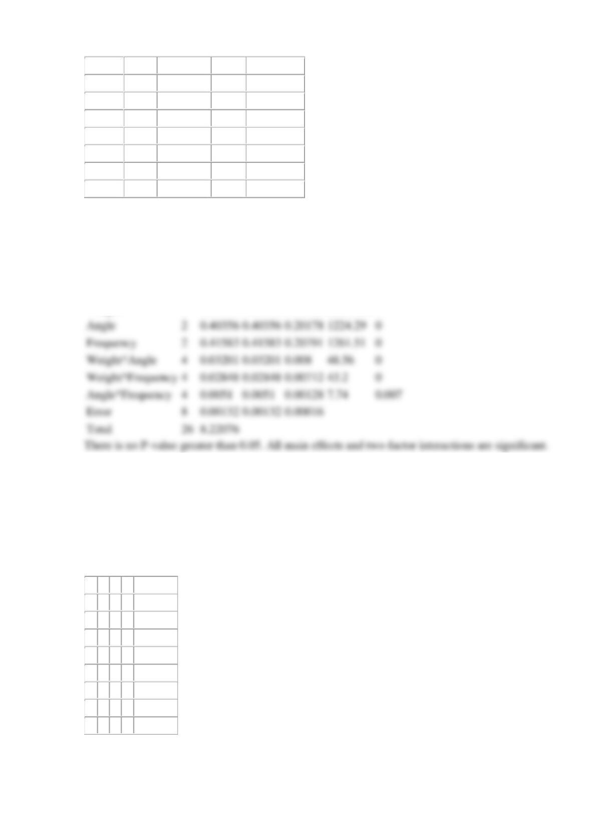
Angle
2
0.40356
0.40356
0.20178
1224.29
0
Frequency
2
0.41583
0.41583
0.20791
1261.51
0
Weight*Angle
4
0.03201
0.03201
0.008
48.56
0
Weight*Frequency
4
0.02848
0.02848
0.00712
43.2
0
Angle*Frequency
4
0.0051
0.0051
0.00128
7.74
0.007
Error
8
0.00132
0.00132
0.00016
Total
26
8.22076
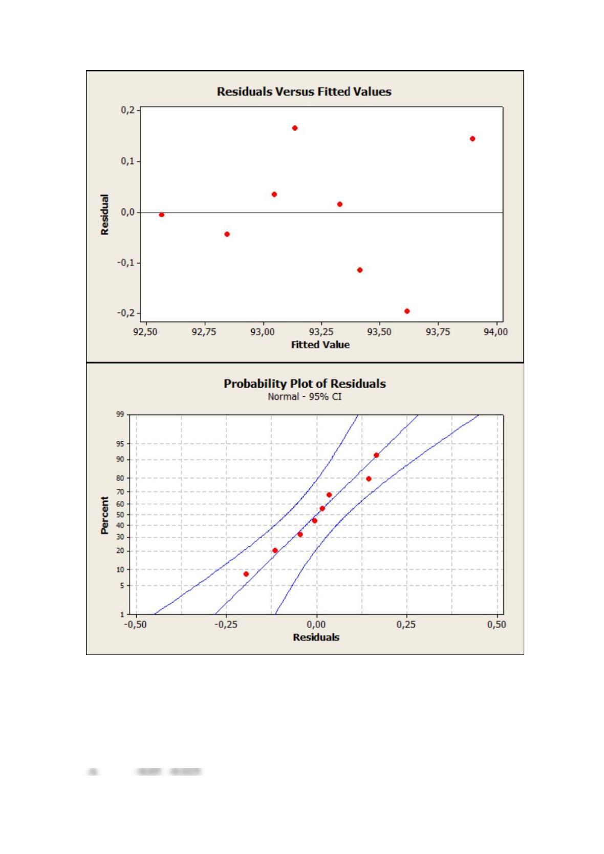
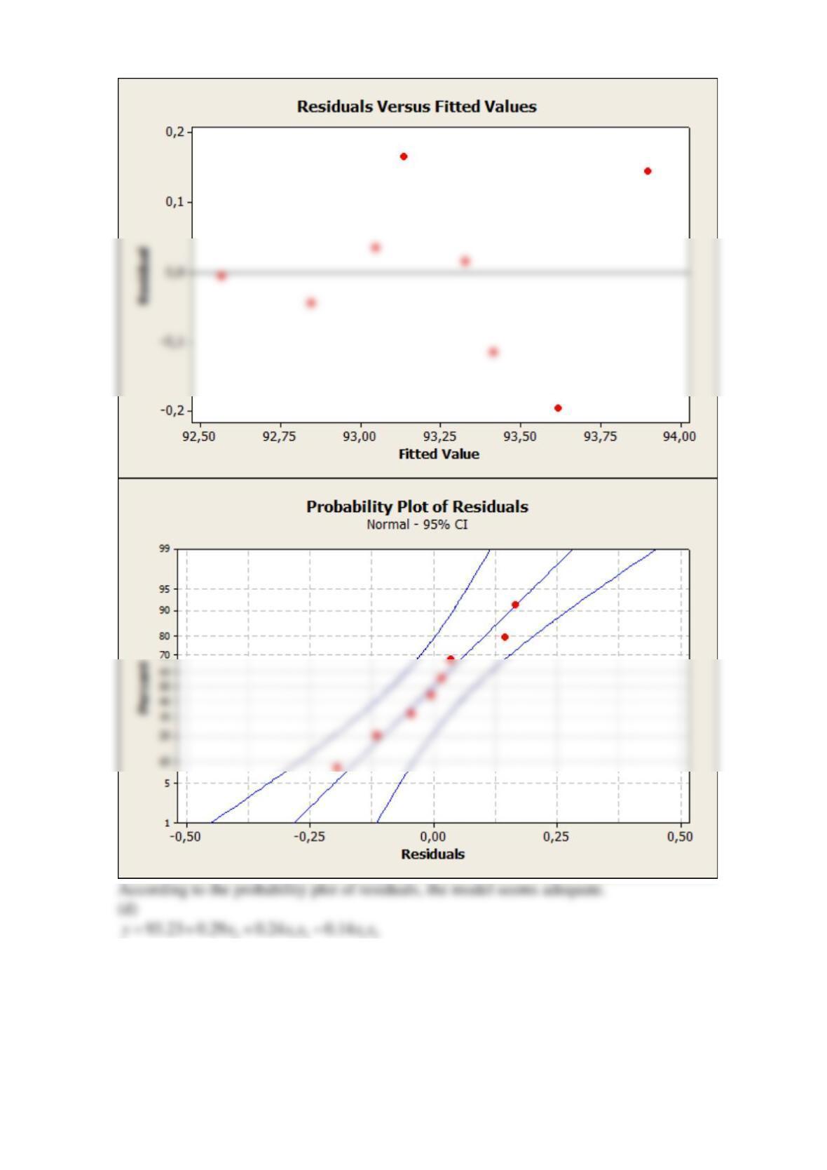
(c) Analyze the residuals and comment on the model adequacy.
(d) Find a regression model to predict yield in terms of the coded factor levels.
SOLUTION
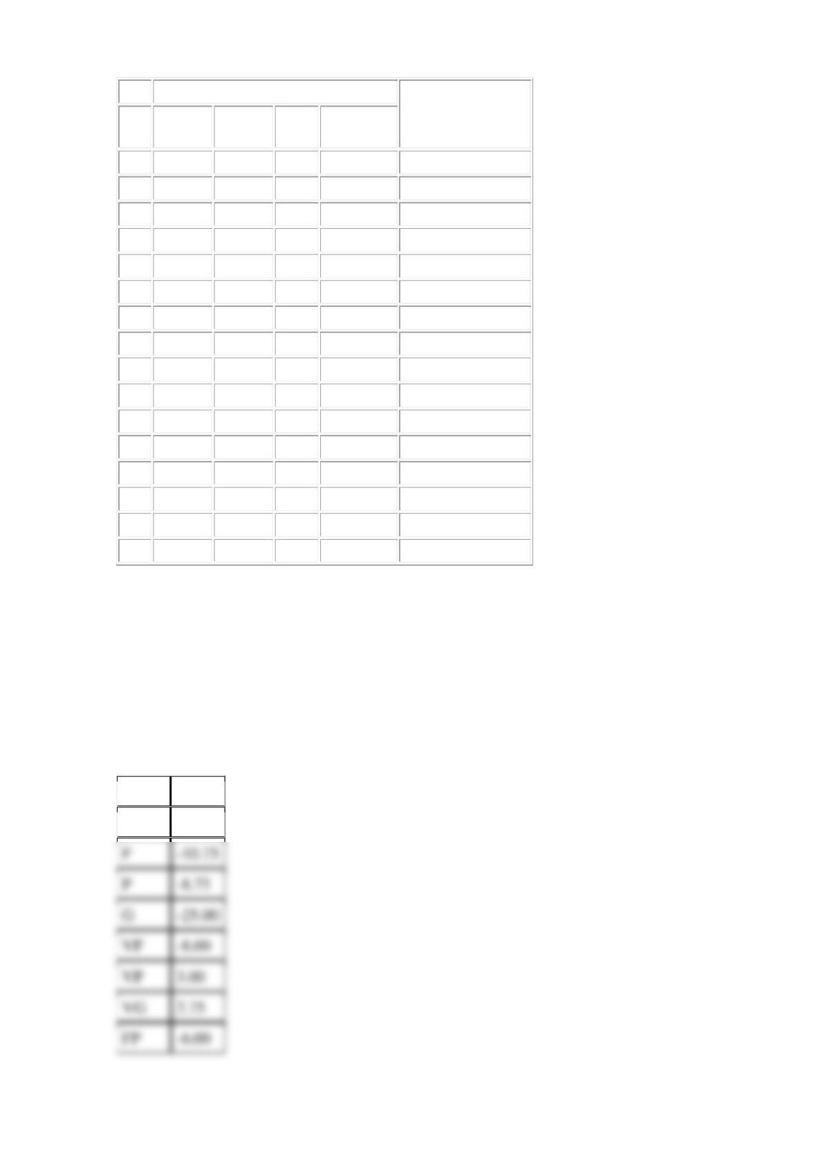
(a)
Term
Effect
Coef
Constant
93.23
A
-0.05
-0.025
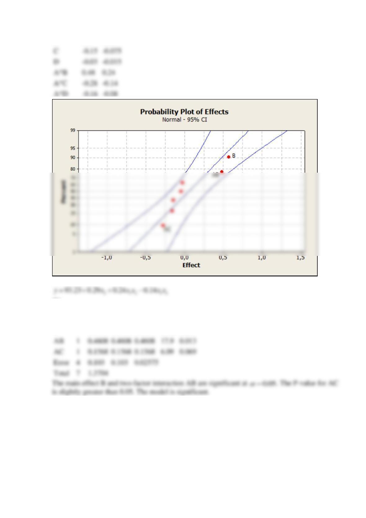
B
0.57
0.285
The model is
(b)
Analysis of Variance for Strength, using Adjusted SS for Tests
Source
DF
Seq SS
Adj SS
Adj MS
F
P
B
1
0.6498
0.6498
0.6498
25.23
0.007
AB
1
0.4608
0.4608
0.4608
17.9
0.013
AC
1
0.1568
0.1568
0.1568
6.09
0.069
Error
4
0.103
0.103
0.02575
Total
7
1.3704
(c)
C
-0.15
-0.075
D
-0.03
-0.015
A*B
0.48
0.24
A*D
-0.16
-0.08
Reserve Supplemental Exercises Chapter 14 Problem 4
An article in the Journal of Manufacturing Systems (1991, vol. 10, pp. 32–40) described an
experiment to investigate the effect of four factors, P = waterjet pressure, F = abrasive flow rate,
G = abrasive grain size, and V = jet traverse speed, on the surface roughness of a waterjet cutter.
A
4
2
design follows.
Factors
Surface Roughness
(μm)
Run
V
(in/min)
F
(lb/min)
P
(kpsi)
G
(Mesh no.)
1
6
2
38
80
104
2
2
2
38
80
98
3
6
2
30
80
103
4
2
2
30
80
96
5
6
1
38
80
137
6
2
1
38
80
112
7
6
1
30
80
143
8
2
1
30
80
129
9
6
2
38
170
88
10
2
2
38
170
70
11
6
2
30
170
110
12
2
2
30
170
110
13
6
1
38
170
102
14
2
1
38
170
76
15
6
1
30
170
98
16
2
1
30
170
68
(a) Estimate the factor effects.
(b) Form a tentative model by examining a normal plot of the effects. Use
0.1
=
.
(c) Find the coefficients for the model in Part B. Use coded units.
(d) Is the model in Parts B and C a reasonable description of the process? What if model includes
main factors only?
(e) Interpret the results of this experiment.
SOLUTION
The estimated effects for the surface roughness:
Term
Effect
V
15.75
F
-10.75
P
-8.75
G
-25.00
-8.00
3.00
FG
19.25
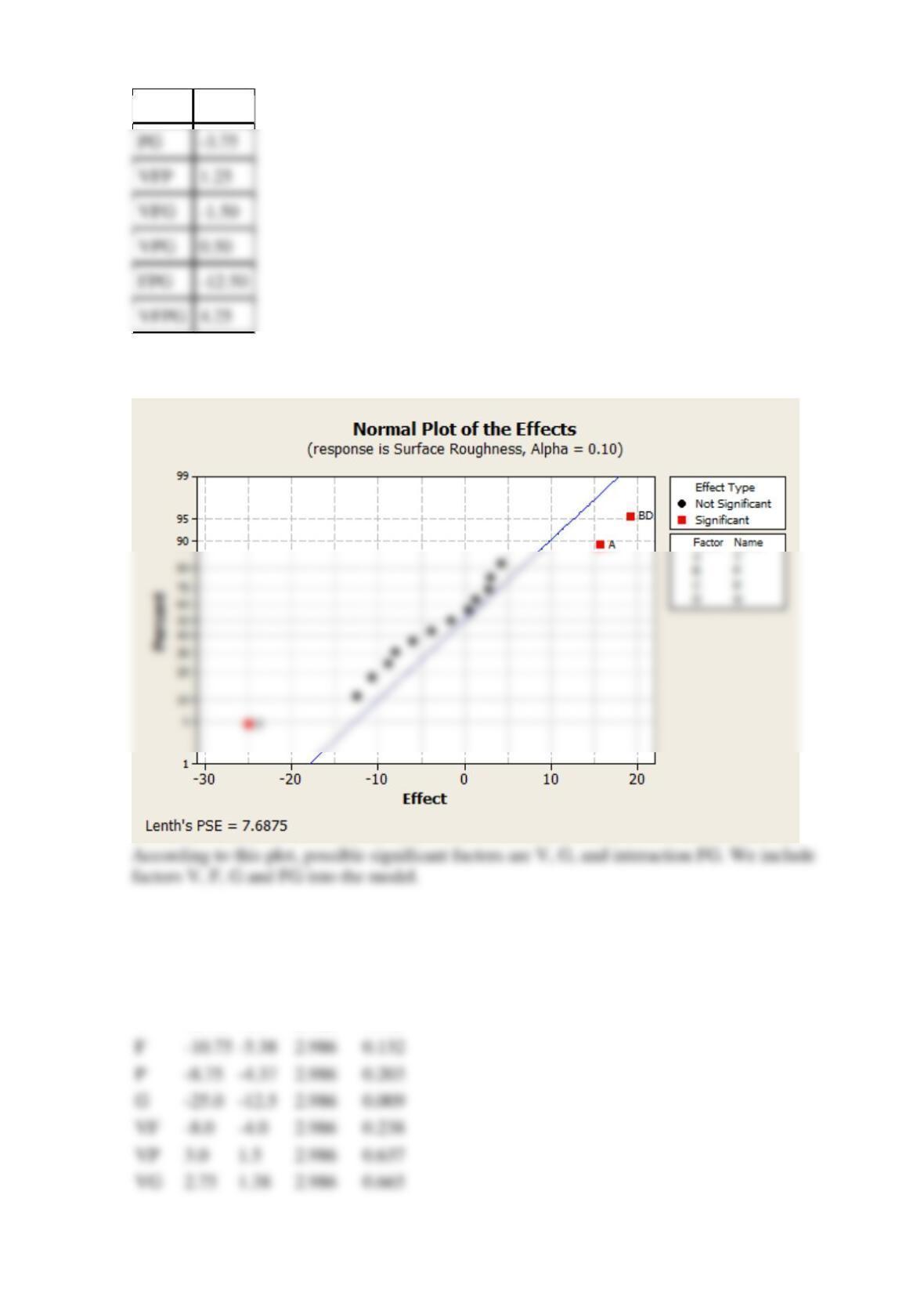
(b)
Plot for the effects:
(c)
Estimated effects and coefficient for surface roughness (coded units):
Term
Effect
Coef
SE Coef
P
Const
102.75
2.986
0
V
15.75
7.87
2.986
0.046
F
-10.75
-5.38
2.986
0.132
P
-8.75
-4.37
2.986
0.203
G
-25.0
-12.5
2.986
0.009
-8.0
-4.0
2.986
0.238
PG
-3.75
VFP
1.25
VFG
-1.50
VPG
0.50
FPG
-12.50
VFPG
4.25
FP
-6.0
-3.0
2.986
0.361
FG
19.25
9.62
2.986
0.023
(d) Is the model in Parts B and C a reasonable description of the process? What if model includes
main factors only?
Analysis of variance for the surface roughness (coded units, only included to model):
Source
DF
SeqSS
AdjSS
AdjMS
F
P
V
1
992.25
992.25
992.25
7.1
0.022
F
1
462.25
462.25
462.25
3.3
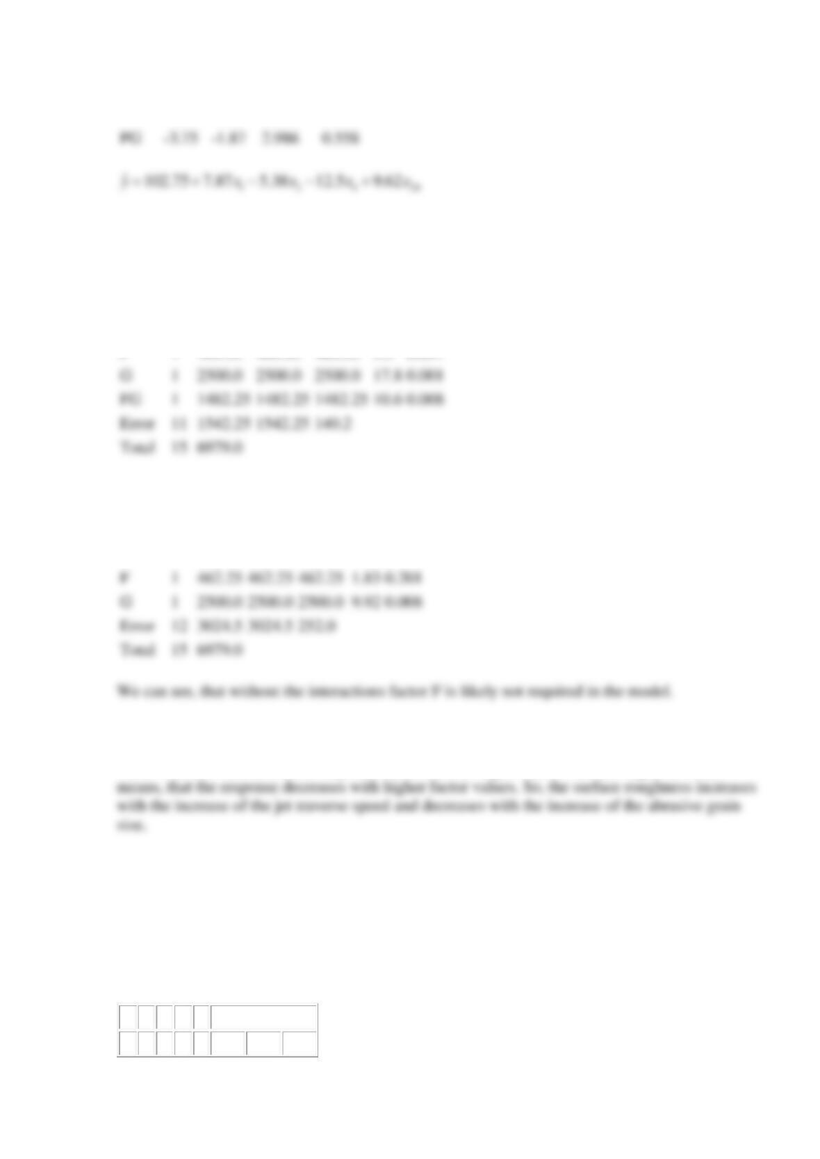
0.097
G
1
2500.0
2500.0
2500.0
17.8
0.001
FG
1
1482.25
1482.25
1482.25
10.6
0.008
Error
11
1542.25
1542.25
140.2
Total
15
6979.0
P-values shows, that the chosen factors are significant, so the model looks reasonable.
Analysis of variance for the surface roughness (coded units, without interactions):
Source
DF
SeqSS
AdjSS
AdjMS
F
P
V
1
992.25
992.25
992.25
3.94
0.071
F
1
462.25
462.25
462.25
1.83
0.201
G
1
2500.0
2500.0
2500.0
9.92
0.008
Error
12
3024.5
3024.5
252.0
Total
15
6979.0
(e)
Positive effect means, that the response increases with higher factor values. Negative effect
Reserve Supplemental Exercises Chapter 14 Problem 5
An article in the Journal of Quality Technology (1985, Vol. 17, pp. 198–206) described the use
of a replicated fractional factorial to investigate the effect of five factors on the free height of leaf
springs used in an automotive application. The factors are A = furnace temperature, B = heating
time, C = transfer time, D = hold down time, and E = quench oil temperature. The data are
shown in the following table.
A
B
C
D
E
Free Height
–
–
–
–
–
7.78
7.78
7.81
PG
-3.75
-1.87
2.986
0.558
+
–
–
+
–
8.15
8.18
7.88
–
+
–
+
–
7.5
7.56
7.5
+
+
–
–
–
7.59
7.56
7.75
–
–
+
+
–
7.54
8.00
7.88
+
–
+
–
–
7.69
8.09
8.06
–
+
+
–
–
7.56
7.52
7.44
+
+
+
+
–
7.56
7.81
7.69
–
–
–
–
+
7.5
7.56
7.5
+
–
–
+
+
7.88
7.88
7.44
–
+
–
+
+
7.5
7.56
7.5
+
+
–
–
+
7.63
7.75
7.56
–
–
+
+
+
7.32
7.44
7.44
+
–
+
–
+
7.56
7.69
7.62
–
+
+
–
+
7.18
7.18
7.25
+
+
+
+
+
7.81
7.5
7.59
(a) What is the generator for this fraction?
(b) Analyze the data. What factors (and interactions) influence the free height? Use
0.05
=
.
(c) Calculate the range of free height for each run. Do any factors affect variability in free
height?
SOLUTION
(a)
The generator for this fraction was I = ABCD.
Alias Structure
I = ABCD
A = BCD
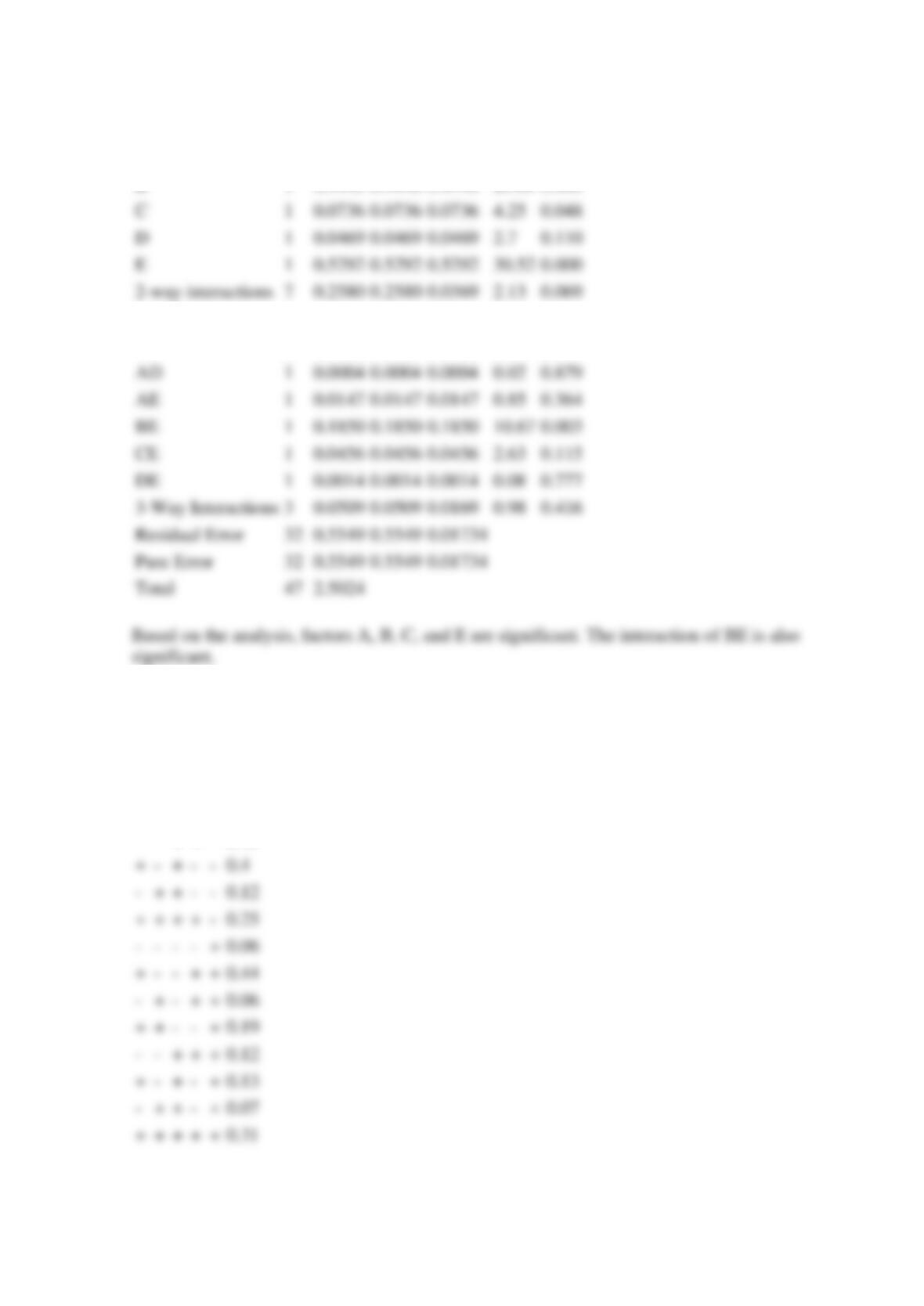
(b) Analysis of Variance for Free Height:
Source
DF
SeqSS
AdjSS
AdjMS
F
P
Main Effects
5
1.6405
1.6405
0.3281
18.92
0.000
A
1
0.5461
0.5461
0.5461
31.5
0.000
B
1
0.4448
0.4448
0.4448
25.65
0.000
AB
1
0.0000
0.0000
0.0000
0.00
0.983
AC
1
0.0108
0.0108
0.0108
0.062
0.463
AD
1
0.0004
0.0004
0.0004
0.02
0.879
AE
1
0.0147
0.0147
0.0147
0.85
0.364
BE
1
0.1850
0.1850
0.1850
10.67
0.003
CE
1
0.0456
0.0456
0.0456
2.63
0.115
DE
1
0.0014
0.0014
0.0014
0.08
0.777
3-Way Interactions
3
0.0509
0.0509
0.0169
0.98
0.416
Residual Error
32
0.5549
0.5549
0.01734
Pure Error
32
0.5549
0.5549
0.01734
Total
47
2.5024
(c) Ranges and factors:
A
B
C
D
E
Range
–
–
–
–
–
0.03
+
–
–
+
–
0.3
–
+
–
+
–
0.06
+
+
–
–
–
0.19
–
–
+
+
–
0.46
+
–
+
–
–
0.4
–
+
+
–
–
0.12
+
+
+
+
–
0.25
–
–
–
–
+
0.06
+
–
–
+
+
0.44
–
+
–
+
+
0.06
+
+
–
–
+
0.19
–
–
+
+
+
0.12
+
–
+
–
+
0.13
–
+
+
–
+
0.07
+
+
+
+
+
0.31
Analysis of variance for range:
D
1
0.0469
0.0469
0.0469
2.7
0.110
E
1
0.5292
0.5292
0.5292
30.52
0.000
2-way interactions
7
0.2580
0.2580
0.0369
2.13
0.069