Applied Statistics and Probability for Engineers, 7th edition 2017
14-41
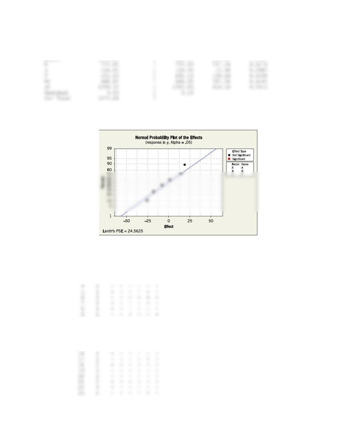
In this model with blocking there are no significant factors.
14.8.5 An article in Quality Engineering [“Designed Experiment to Stabilize Blood Glucose Levels” (1999–2000,
Vol. 12, pp. 83–87)] reported on an experiment to minimize variations in blood glucose levels. The factors were
volume of juice intake before exercise (4 or 8 oz), amount of exercise on a Nordic Track cross-country skier (10 or 20
min), and delay between the time of juice intake (0 or 20 min) and the beginning of the exercise period. The experiment
was blocked for time of day. The data follow.
(a) What effects are confounded with blocks? Comment on any concerns with the confounding in this design.
(b) Analyze the data and draw conclusions.
Run
Juice (oz)
Exercise (min)
Delay (min)
Time of Day
Average Blood
Glucose
1
4
10
0
pm
71.5
2
8
10
0
am
103
3
4
20
0
am
83.5
4
8
20
0
pm
126
5
4
10
20
am
125.5
6
8
10
20
pm
129.5
7
4
20
20
pm
95
8
8
20
20
am
93
Factorial Fit: y versus Block, A, B, C
Estimated Effects and Coefficients for y (coded units)
Term Effect Coef
Constant 103.38
B -8.00 -4.00
A*B 1.25 0.62
Applied Statistics and Probability for Engineers, 7th edition 2017
14-42
Sum of Mean F
Source Squares DF Square Value Prob > F
Block 36.13 1 36.13
Thus, the effects of juice as well as the interactions between juice and delay and exercise and delay were marginally significant.
Additional degrees of freedom for error are needed and the normal probability plot of the effects does not indicate significant
effects.
14.8.6 Consider the 26 factorial design. Set up a design to be run in four blocks of 16 runs each. Show that a design that
confounds three of the four-factor interactions with blocks is the best possible blocking arrangement.
26 in 4 blocks.
Run Block A B C D E F
1 1 – – – + + –
2 1 + – + + – –
3 1 – + – – + +
10 1 + + – – – –
11 1 – + + – + –
12 1 + – – – + +
13 1 – – – – – –
14 1 – + – + – +
15 1 + + + + + +

Applied Statistics and Probability for Engineers, 7th edition 2017
14-43
24 2 – – + + + –
25 2 – – + – – –
26 2 + – + – + +
37 3 – + – – – +
38 3 – – + + – +
39 3 + – – + + +
40 3 + – + + + –
41 3 + – + – – –
52 4 – – + + – –
53 4 – + + + + +
54 4 – + – – – –
55 4 + – + – – +
56 4 + + – + – +
14.8.7 An article in Advanced Semiconductor Manufacturing Conference (ASMC) (May 2004, pp. 325–29) stated that
dispatching rules and rework strategies are two major operational elements that impact productivity in a semiconductor
fabrication plant (fab). A four-factor experiment was conducted to determine the effect of dispatching rule time (5 or 10
min), rework delay (0 or 15 min), fab temperature (60 or 80°F), and rework levels (level 0 or level 1) on key fab
performance measures. The performance measure that was analyzed was the average cycle time. The experiment was
blocked for the fab temperature. Data modified from the original study are in the following table.
Run
Dispatching
Rule Time
(min)
Rework Delay
(min)
Rework Level
Fab
Temperature
(°F)
Average Cycle
Time Run
(min)
1
5
0
0
60
218
2
10
0
0
80
256.5
3
5
0
1
80
231
4
10
0
1
60
302.5
5
5
15
0
80
298.5
6
10
15
0
60
314
7
5
15
1
60
249
Applied Statistics and Probability for Engineers, 7th edition 2017
14-44
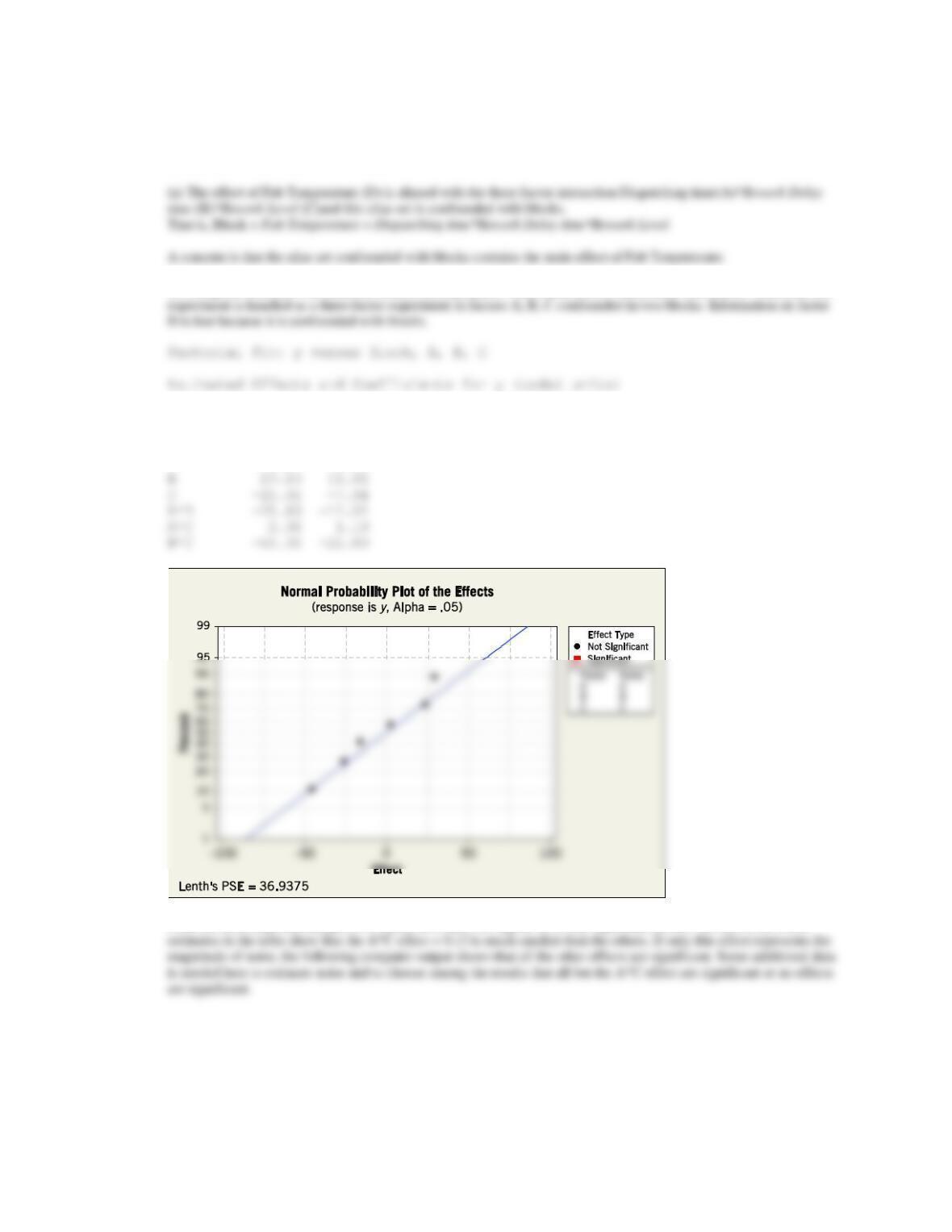
(a) What effects are confounded with blocks? Do you find any concerns with confounding in this design? If so,
comment on it.
(b) Analyze the data and draw conclusions.
(b) Computer software will often not analyze an experiment with a main effect confounded with blocks. Therefore, the
Term Effect Coef
Constant 263.81
Block 7.06
A 29.37 14.69
From the normal probability plot of effects, there does not appear to be any significant effects. However, the effect
Applied Statistics and Probability for Engineers, 7th edition 2017
14-45
Factorial Fit: y versus Block, A, B, C
Estimated Effects and Coefficients for y (coded units)
Term Effect Coef SE Coef T P
Constant 263.81 1.188 222.16 0.003
Block 7.06 1.188 5.95 0.106
Analysis of Variance for y (coded units)
Source DF Seq SS Adj SS Adj MS F P
Blocks 1 399.03 399.03 399.03 35.37 0.106
Section 14.9
14.9.1 An article by L. B. Hare [“In the Soup: A Case Study to Identify Contributors to Filling Variability,” Journal of Quality
Technology 1988 (Vol. 20, pp. 36–43)] described a factorial experiment used to study filling variability of dry soup mix
packages. The factors are A = number of mixing ports through which the vegetable oil was added (1, 2), B =
temperature surrounding the mixer (cooled, ambient), C = mixing time (60, 80 s), D = batch weight (1500, 2000 lb),
and E = number of days of delay between mixing and packaging (1, 7). Between 125 and 150 packages of soup were
sampled over an 8-hour period for each run in the design, and the standard deviation of package weight was used as the
response variable. The design and resulting data follow.
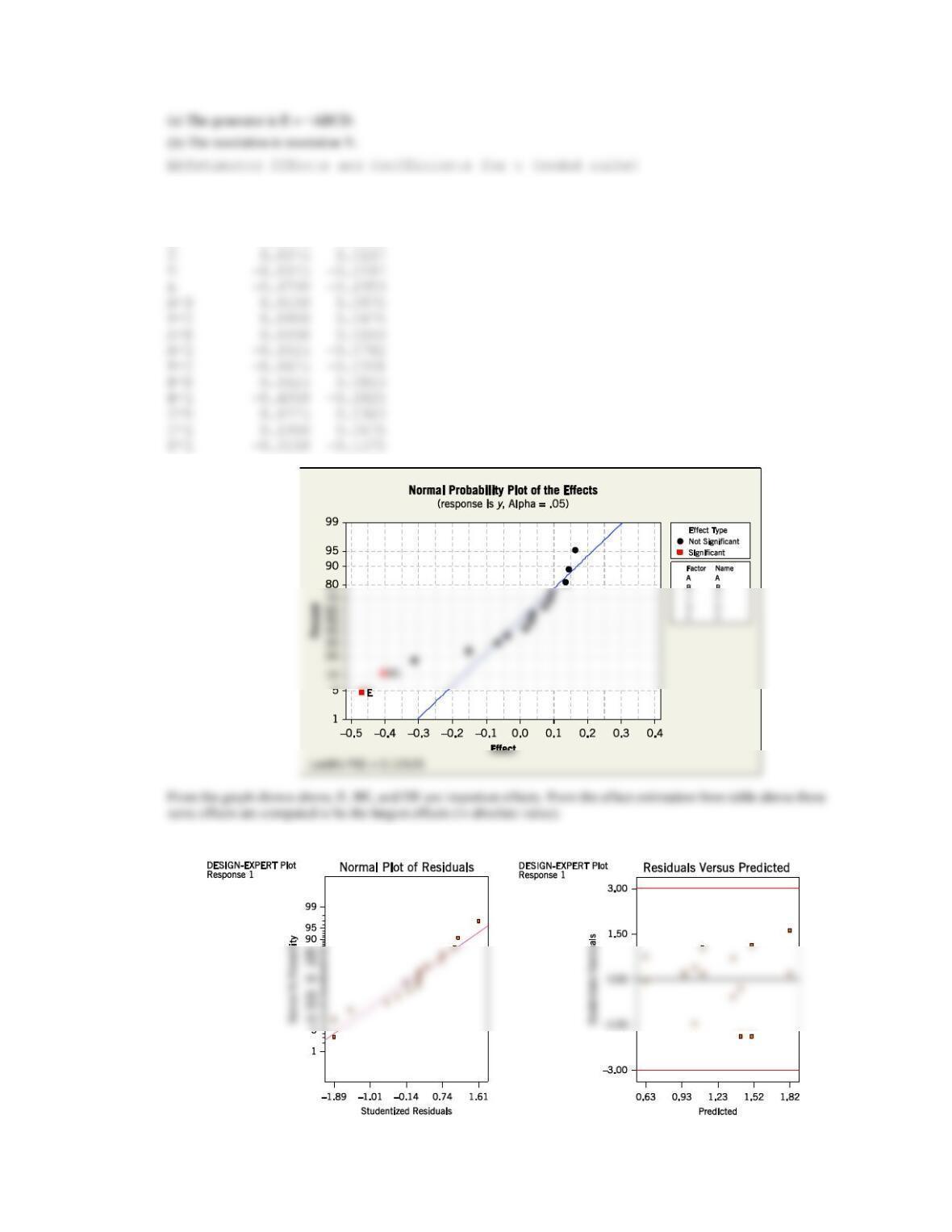
(a) What is the generator for this design?
(b) What is the resolution of this design?
(c) Estimate the factor effects. Which effects are large?
(d) Does a residual analysis indicate any problems with the underlying assumptions?
(e) Draw conclusions about this filling process.
Std Order
A
Mixer Ports
B Temp
C Time
D Batch
Weight
E Delay
y Std Dev
1
−
−
−
−
−
1.13
2
+
−
−
−
+
1.25
3
−
+
−
−
+
0.97
4
+
+
−
−
−
1.70
5
−
−
+
−
+
1.47
6
+
−
+
−
−
1.28
7
−
+
+
−
−
1.18
8
+
+
+
−
+
0.98
9
−
−
−
+
+
0.78
10
+
−
−
+
−
1.36
11
−
+
−
+
−
1.85
12
+
+
−
+
+
0.62
13
−
−
+
+
−
1.09
14
+
−
+
+
+
1.10
15
−
+
+
+
+
0.76
16
+
+
+
+
−
2.10
Applied Statistics and Probability for Engineers, 7th edition 2017
14-46
Term Effect Coef
Constant 1.2263
A 0.1450 0.0725
B 0.0875 0.0438
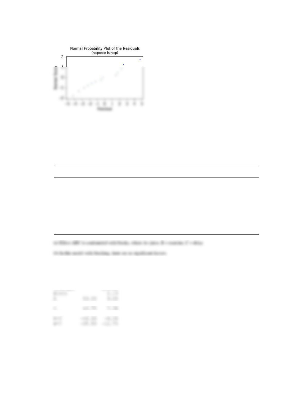
(d) For the model with E, BE, and DE the normality assumption and constant variance seem to be reasonable.
Applied Statistics and Probability for Engineers, 7th edition 2017
14-47
Analysis of variance table [Partial sum of squares]
Source Sum of Mean F
Model Squares DF Square Value Prob > F
1.97 5 0.39 8.94 0.0019
B 0.031 1 0.031 0.69 0.4242
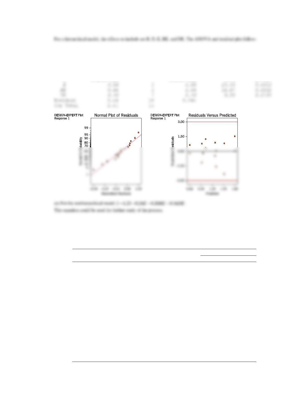
14.9.2 An article in Quality Engineering [“A Comparison of Multi-Response Optimization: Sensitivity to Parameter
Selection” (1999, Vol. 11, pp. 405–415)] conducted a half replicate of a 25 factorial design to optimize the retort
process of beef stew MREs, a military ration. The design factors are x1 = sauce viscosity, x2 = residual gas,
x3 = solid/liquid ratio, x4 = net weight, x5 = rotation speed. The response variable is the heating rate index, a measure of
heat penetration, and there are two replicates.
Run
x1
x2
x3
x4
x5
Heating Rate Index
I
II
1
−1
−1
−1
−1
1
8.46
9.61
2
1
−1
−1
−1
−1
15.68
14.68
3
−1
1
−1
−1
−1
14.94
13.09
4
1
1
−1
−1
1
12.52
12.71
5
−1
−1
1
−1
−1
17.0
16.36
6
1
−1
1
−1
1
11.44
11.83
7
−1
1
1
−1
1
10.45
9.22
8
1
1
1
−1
−1
19.73
16.94
9
−1
−1
−1
1
−1
17.37
16.36
10
1
−1
−1
1
1
14.98
11.93
11
−1
1
−1
1
1
8.40
8.16
12
1
1
−1
1
−1
19.08
15.40
13
−1
−1
1
1
1
13.07
10.55
14
1
−1
1
1
−1
18.57
20.53
15
−1
1
1
1
−1
20.59
21.19
16
1
1
1
1
1
14.03
11.31
Applied Statistics and Probability for Engineers, 7th edition 2017
14-48
(a) Estimate the factor effects. Based on a normal probability plot of the effect estimates, identify a model for the data
from this experiment.
(b) Conduct an ANOVA based on the model identified in part (a). What are your conclusions?
(c) Analyze the residuals and comment on model adequacy.
(d) Find a regression model to predict yield in terms of the coded factor levels.
(e) This experiment was replicated, so an ANOVA could have been conducted without using a normal plot of the
Effects to tentatively identify a model. What model would be appropriate? Use the ANOVA to analyze this model and
compare the results with those obtained from the normal probability plot approach.
(a) Estimated Effects and Coefficients for Heat (coded units)
Term Effect Coef SE Coef T P
Constant 14.256 0.2370 60.15 0.000
A 1.659 0.829 0.2370 3.50 0.003
B -0.041 -0.021 0.2370 -0.09 0.932
D 1.679 0.839 0.2370 3.54 0.003
A*B 0.301 0.151 0.2370 0.64 0.534
A*C -0.915 -0.457 0.2370 -1.93 0.071
Applied Statistics and Probability for Engineers, 7th edition 2017
14-49
(b)
Analysis of variance table [Partial sum of squares]
Source Sum of Mean
Model Squares DFSquare FValue Prob > F
399.85 6 66.64 31.03 < 0.0001
A 22.01 1 22.01 10.25 0.0037
C 27.08 1 27.08 12.61 0.0016
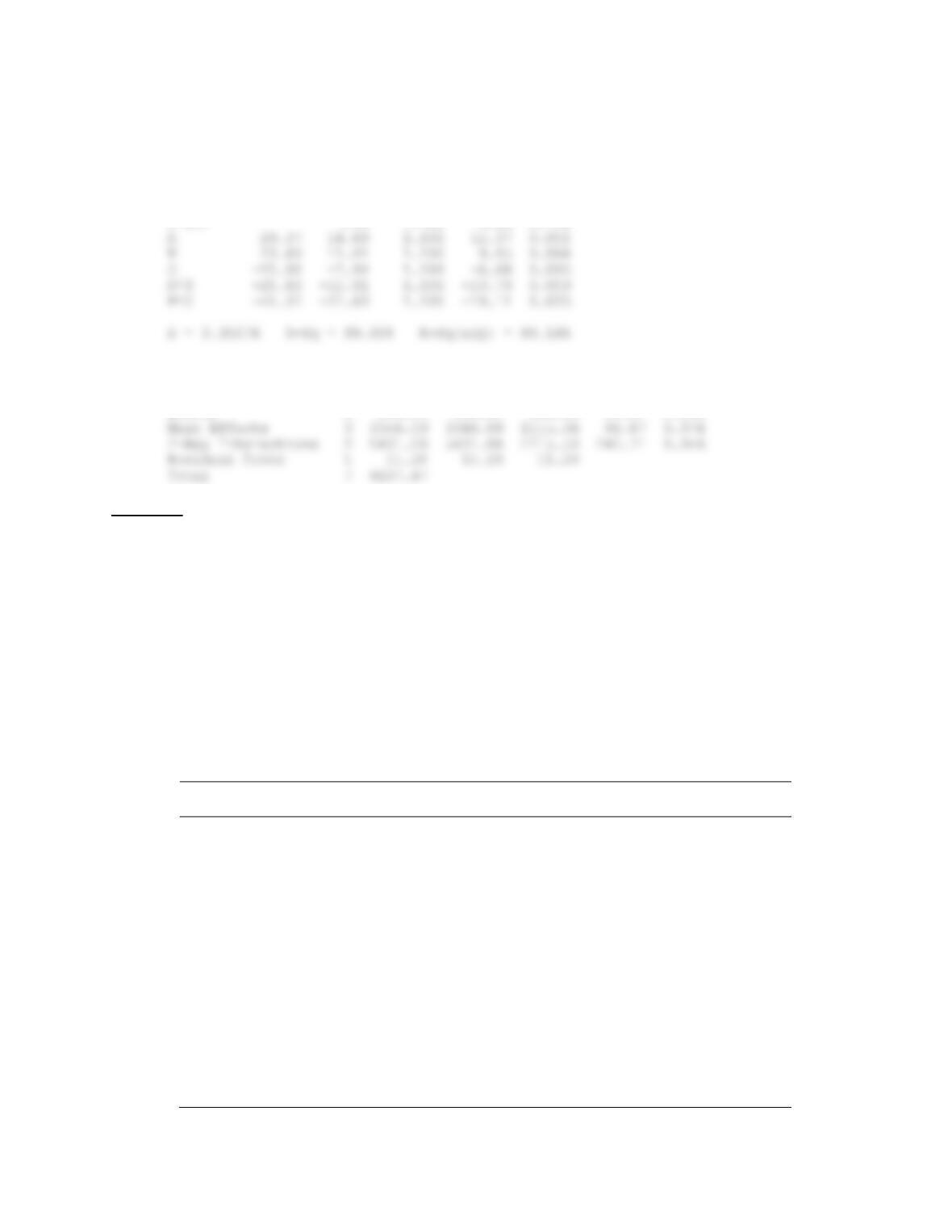
(c) The residual plots do not show any violations of the assumptions.
(e) Use the t-test to test individual effects as shown below
Term Effect Coef SE Coef T P
Constant 14.256 0.2370 60.15 0.000
A 1.659 0.829 0.2370 3.50 0.003
B -0.041 -0.021 0.2370 -0.09 0.932
At
Applied Statistics and Probability for Engineers, 7th edition 2017
14-50
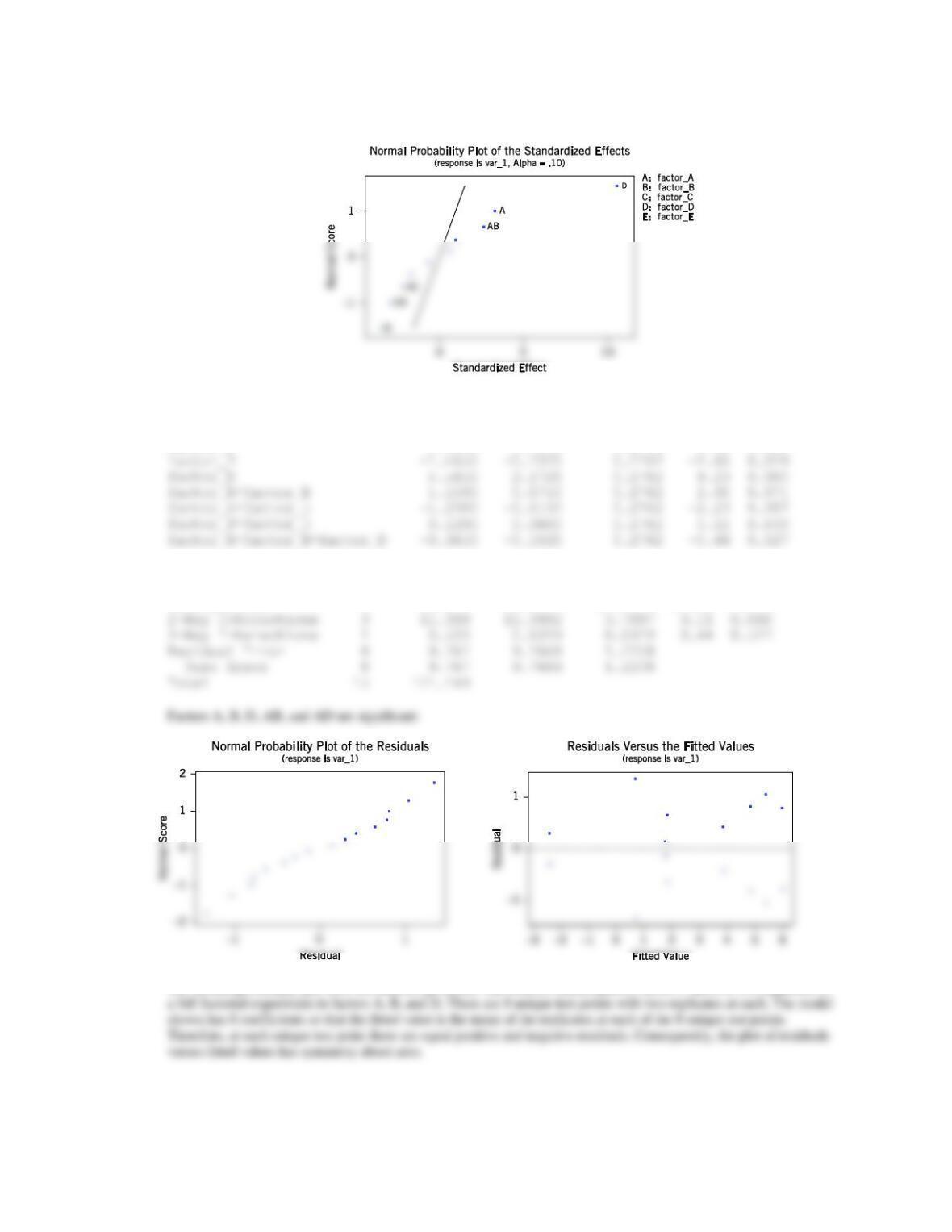
14.9.3 R. D. Snee (“Experimenting with a Large Number of Variables,” in Experiments in Industry: Design, Analysis and
Interpretation of Results, Snee, Hare, and Trout, eds., ASQC, 1985) described an experiment in which a 25–1 design
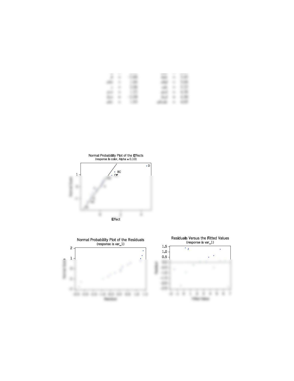
with I = ABCDE was used to investigate the effects of five factors on the color of a chemical product.
The factors are A = solvent/reactant, B = catalyst/reactant, C = temperature, D = reactant purity, and
E = reactant pH. The results obtained are as follows:
e
=
−0.63
d
=
6.79
(a) Prepare a normal probability plot of the effects. Which factors are active?
(b) Calculate the residuals. Construct a normal probability plot of the residuals and plot the residuals versus the fitted
values. Comment on the plots.
(c) If any factors are negligible, collapse the 25–1 design into a full factorial in the active factors. Comment on the
resulting design, and interpret the results.
(a) Several factors and interactions are potentially significant.
(b) There are no serious problems with the residual plots. The normal probability plot has some curvature and there is a
little more variability at the lower and higher ends of the fitted values.
=
−2.68
=
3.45
=
=
5.22
=
−2.09
=
4.30
Applied Statistics and Probability for Engineers, 7th edition 2017
14-51
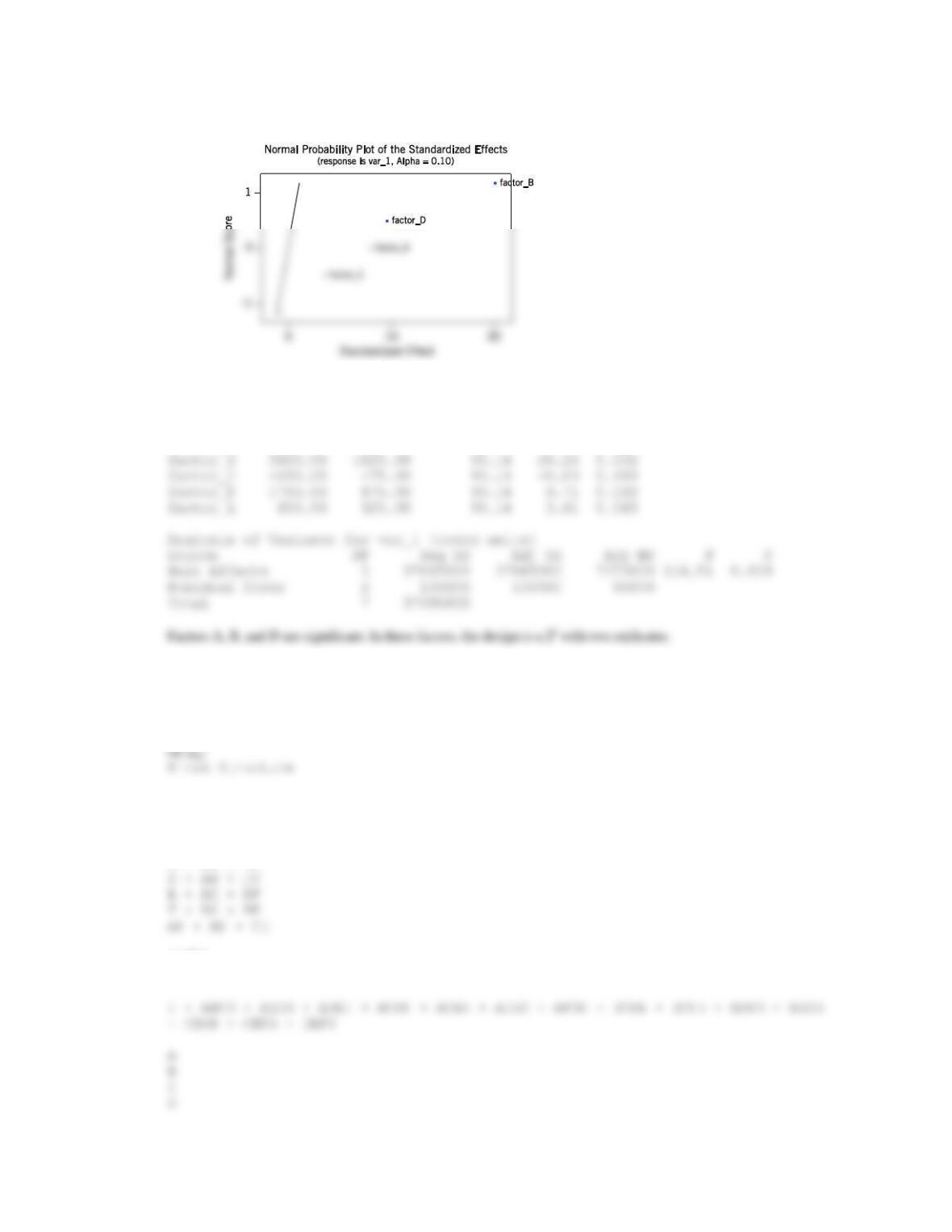
(c) Normal probability plot shows that we can collapse using only factors A, B, and D.
Estimated Effects and Coefficients for var_1
Term Effect Coef StDev Coef T P
Constant 2.7700 0.2762 10.03 0.000
factor_A 1.4350 0.7175 0.2762 2.60 0.032
Analysis of Variance for var_1
Source DF Seq SS Adj SS Adj MS F P
Main Effects 3 99.450 99.4499 33.1500 27.15 0.000
The normal probability plot does not indicate problems. The reduced model ignores factor C and it is two replicates of
Applied Statistics and Probability for Engineers, 7th edition 2017
14-52
Section 14.10
14.10.1 An article in Industrial and Engineering Chemistry [“More on Planning Experiments to Increase Research Efficiency”
(1970, pp. 60–65)] uses a 25−2 design to investigate the effect on process yield of A = condensation temperature, B =
amount of material 1, C = solvent volume, D = condensation time, and E = amount of material 2. The results obtained
are as follows:
ae
=
23.2
cd
=
23.8
ab
=
15.5
ace
=
23.4
(a) Verify that the design generators used were I = ACE and I = BDE.
(b) Write down the complete defining relation and the aliases from the design.
(c) Estimate the main effects.
(d) Prepare an analysis of variance table. Verify that the AB and AD interactions are available to use as error.
(e) Plot the residuals versus the fitted values. Also construct a normal probability plot of the residuals. Comment on the
results.
(a)The design generators are I=ACE and I=BDE. This is verified by looking at the following table.
The contrast for E is calculated using E=AC and the contrast for D is calculated using D=BE.
A
B
C
D
E
Response
−1
−1
−1
−1
1
23.2
1
1
16.9
−1
1
1
−1
−1
16.2
1
1
1
23.4
−1
1
−1
1
1
16.8
(b) Design Generator: D = BE, E = AC
Aliases
A = CE = BCDE = ABDE
B = DE = ACDE = ABCE
(c) Estimated Effects and Coefficients for response (coded units)
Term Effect Coef SE Coef T P
Constant 19.238 0.7871 24.44 0.002
A -1.525 -0.762 0.7871 -0.97 0.435
=
16.9
=
16.8
bc
=
16.2
abcde
=
18.1
Applied Statistics and Probability for Engineers, 7th edition 2017
14-53
(d) Estimated Effects and Coefficients for response (coded units)
Term Effect Coef SE Coef T P
Constant 19.238 1.138 16.91 0.038
A -1.525 -0.762 1.138 -0.67 0.624
B -5.175 -2.587 1.138 -2.27 0.264
Analysis of Variance for response (coded units)
Source DF Seq SS Adj SS Adj MS F P
Main Effects 4 69.475 69.475 17.369 1.68 0.517
(e) The normal probability plot and the plot of the residuals versus fitted values are satisfactory.
14.10.2 Suppose that in Exercise 14.6.2 only a
14
fraction of the 25 design could be run. Construct the design and analyse the
data that are obtained by selecting only the response for the eight runs in your design.
Generators D = AB, E = AC for 25−2, Resolution III
A
B
C
D
E
var_1
−1
−1
−1
1
1
1900
1
−1
−1
−1
−1
900
−1
1
−1
−1
1
3500
1
1
−1
1
−1
6100
−1
−1
1
1
−1
800
1
−1
1
−1
1
1200
−1
1
1
−1
−1
3000
Applied Statistics and Probability for Engineers, 7th edition 2017
14-54
The normal probability plot and table below show that factors A, B, and D are significant.
Estimated Effects and Coefficients for var_1 (coded units)
Term Effect Coef SE Coef T P
Constant 3025.00 90.14 33.56 0.001
factor_A 1450.00 725.00 90.14 8.04 0.015
14.10.3 For each of the following designs, write down the aliases, assuming that only main effects and two factor interactions
are of interest.
(a)
−63
III
2
(b)
−84
IV
2
III
2
−63
I + ABD + ACE + BCF + DEF + ABEF + ACDF + BCDE
A + BD + CE
B + AD + CF
C + AE + BF
(b)
−84
IV
2
Alias Structure
Applied Statistics and Probability for Engineers, 7th edition 2017
14-55
E
F
G
14.10.4 Consider the 26−2 design in Table 14.26.
(a) Suppose that after analyzing the original data, we find that factors C and E can be dropped. What type of
2k design is left in the remaining variables?
(b) Suppose that after the original data analysis, we find that factors D and F can be dropped. What type of
2k design is left in the remaining variables? Compare the results with part (a). Can you explain why the answers are
different?
(a) Because factors A, B, C, and E form a word in the complete defining relation, it can be verified that the resulting
14.10.5 An article in the Journal of Marketing Research (1973, Vol. 10(3), pp. 270–276) presented a 27−4 fractional factorial
design to conduct marketing research:
Runs
A
B
C
D
E
F
G
Sales for a 6-Week Period (in
$1000)
1
−1
−1
−1
1
1
1
−1
8.7
2
1
−1
−1
−1
−1
1
1
15.7
3
−1
1
−1
−1
1
−1
1
9.7
4
1
1
−1
1
−1
−1
−1
11.3
5
−1
−1
1
1
−1
−1
1
14.7
6
1
−1
1
−1
1
−1
−1
22.3
7
−1
1
1
−1
−1
1
−1
16.1
8
1
1
1
1
1
1
1
22.1
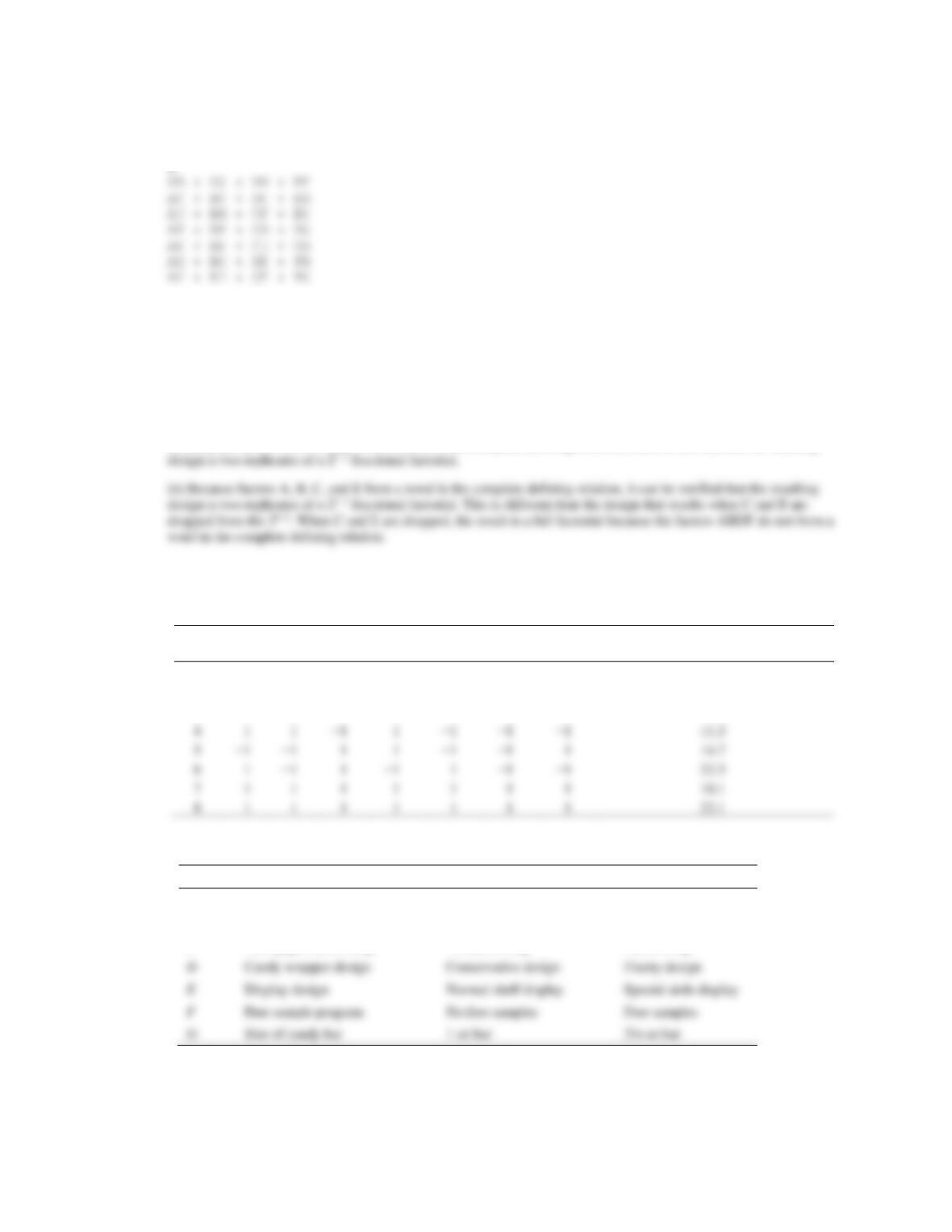
The factors and levels are shown in the following table.
Factor
−1
+1
A
Television advertising
No advertising
Advertising
B
Billboard advertising
No advertising
Advertising
C
Newspaper advertising
No advertising
Advertising
Candy wrapper design
Conservative design
Flashy design
E
Display design
Normal shelf display
Special aisle display
F
Free sample program
No free samples
Free samples
Size of candy bar
1 oz bar
2½ oz bar
(a) Write down the alias relationships.
(b) Estimate the main effects.
Applied Statistics and Probability for Engineers, 7th edition 2017
14-56
(c) Prepare a normal probability plot for the effects and interpret the results.
(a)
Alias Structure (up to order 3)
I + A*B*D + A*C*E + A*F*G + B*C*F + B*E*G + C*D*G + D*E*F
A + B*D + C*E + F*G + B*C*G + B*E*F + C*D*F + D*E*G
(b)
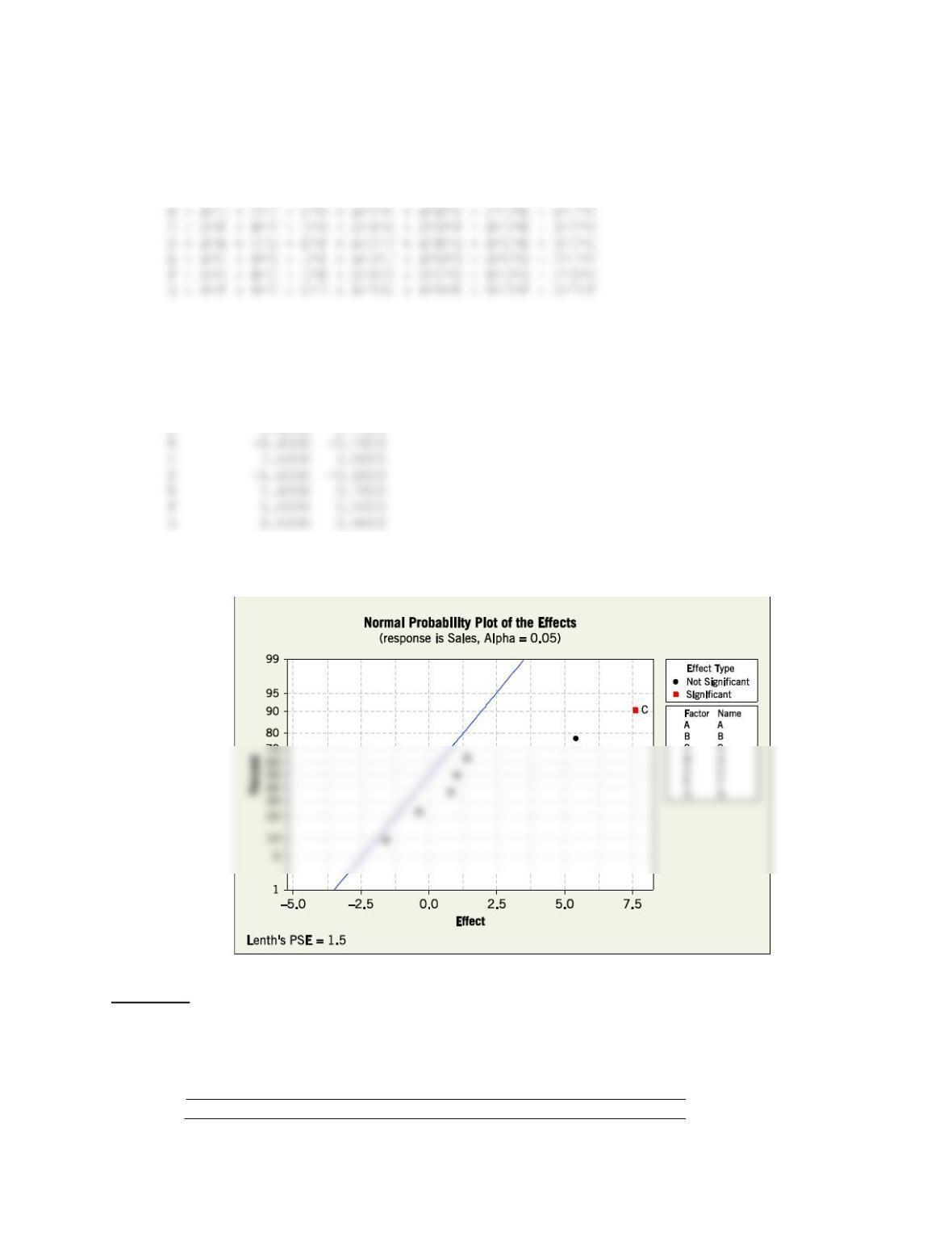
Factorial Fit: Sales Versus A, B, C, D, E, F, G
Estimated Effects and Coefficients for Sales (coded units)
Term Effect Coef
Constant 15.0000
A 5.4000 2.7000
(c) The plot indicates that only Factor C is a significant effect, but one might also consider the effect of A as
sufficiently distant from the line to be considered significant.
Section 14.11
14.11.1 An article in Rubber Age (1961, Vol. 89, pp. 453–458) describes an experiment on the manufacture of a product in
which two factors were varied. The factors are reaction time (hr) and temperature (°C). These factors are coded as x1 =
(time − 12)/8 and x2 = (temperature − 250)/30. The following data were observed where y is the yield (in percent):
Run Number
x1
x2
y
Applied Statistics and Probability for Engineers, 7th edition 2017
14-57
1
−1
0
83.8
2
1
0
81.7
3
0
0
82.4
4
0
0
82.9
5
0
−1
84.7
6
0
1
75.9
7
0
0
81.2
8
−1.414
−1.414
81.3
9
−1.414
1.414
83.1
10
1.414
−1.414
85.3
11
1.414
1.414
72.7
12
0
0
82.0
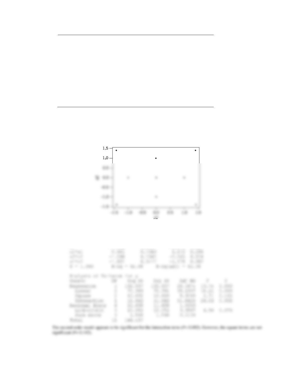
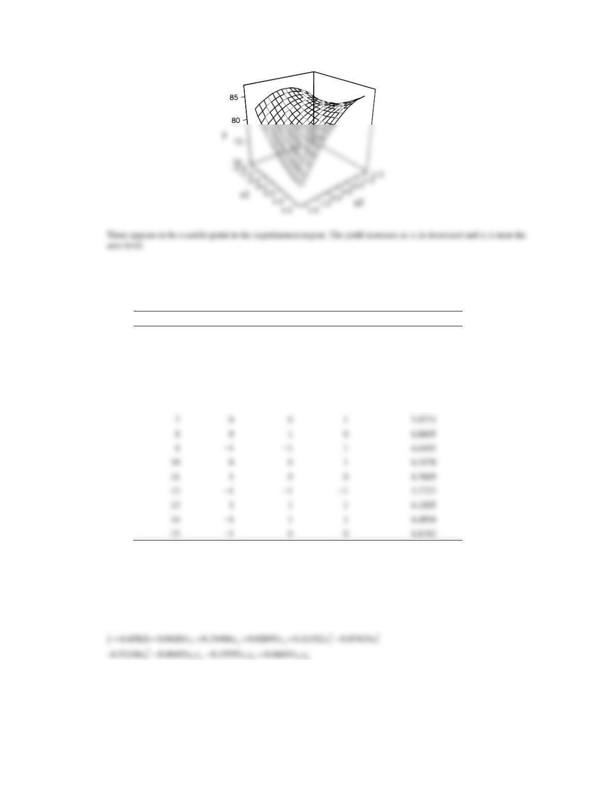
(a) Plot the points at which the experimental runs were made.
(b) Fit a second-order model to the data. Is the second-order model adequate?
(c) Plot the yield response surface. What recommendations would you make about the operating conditions for this
process?
(a)
(b)
Estimated Regression Coefficients for y
Term Coef StDev T P
Constant 82.024 0.5622 145.905 0.000
x1 -1.115 0.4397 -2.536 0.044
x2 -2.408 0.4397 -5.475 0.002
(c)
Applied Statistics and Probability for Engineers, 7th edition 2017
14-58
14.11.2 An article in Quality Engineering [“Mean and Variance Modeling with Qualitative Responses: A Case Study”(1998–
1999, Vol. 11, pp. 141–148)] studied how three active ingredients of a particular food affect the overall taste of the
product. The measure of the overall taste is the overall mean liking score (MLS). The three ingredients are identified by
the variables x1, x2, and x3. The data are shown in the following table.
Run
x1
x2
x3
MLS
1
1
1
−1
6.3261
2
1
1
1
6.2444
3
0
0
0
6.5909
4
0
−1
0
6.3409
5
1
−1
1
5.907
6
1
−1
−1
6.488
8
0
1
0
6.8605
9
−1
−1
1
6.0455
0
0
1
6.3478
1
0
0
6.7609
−1
−1
−1
5.7727
−1
1
−1
6.1805
−1
0
0
6.8182
(a) Fit a second-order response surface model to the data.
(b) Construct contour plots and response surface plots for MLS. What are your conclusions?
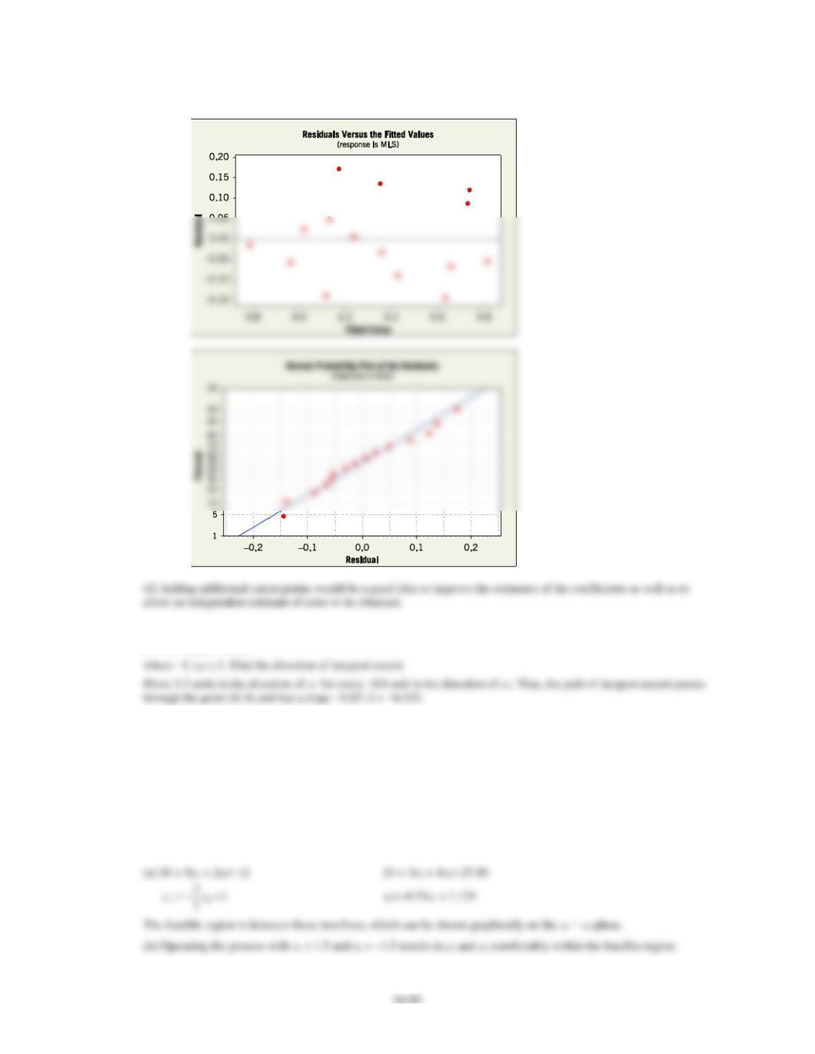
(c) Analyze the residuals from this experiment. Does your analysis indicate any potential problems?
(d) This design has only a single center point. Is this a good design in your opinion?
(a)
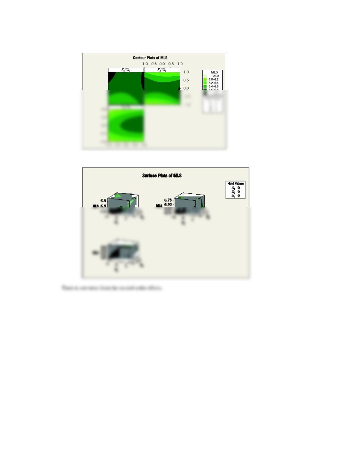
Applied Statistics and Probability for Engineers, 7th edition 2017
14-59
(b) Contour Plots
Response surface plots
Applied Statistics and Probability for Engineers, 7th edition 2017
(c) The residual plots appear reasonable.
14.11.3 Consider the first-order model
= + −
50 1.5 0.8y x x
14.11.4 A manufacturer of cutting tools has developed two empirical equations for tool life (y1) and tool cost (y2). Both models
are functions of tool hardness (x1) and manufacturing time (x2). The equations are
= + +
= + +
1 1 2
2 1 2
10 5 2
23 3 4
y x x
y x x
and both are valid over the range −1.5 ≤ xi ≤ 1.5. Suppose that tool life must exceed 12 hours and cost must be below
$27.50.
(a) Is there a feasible set of operating conditions?
(b) Where would you run this process?